Description and Analysis of Algorithm 002

Learning Requirements

Algorithm Complexity Calculation Methods

Analysis methods for time complexity and space complexity of algorithms.

Algorithm Description and Analysis

【1】

The computation of data is described by algorithms (Algorithm)

Algorithms are an important part of data structure courses.

An algorithm is a well-defined computational process that takes one or more values as input and produces one or more values as output. Therefore, an algorithm is a series of steps that transforms input into output.

In general, an input instance of a problem consists of all the inputs required to compute the solution to that problem, satisfying the constraints given in the problem statement. If an algorithm can terminate and provide a correct result for every input instance, it is called a correct algorithm. A correct algorithm solves the given computational problem.

Of course, there are many algorithms that can solve a problem correctly, but how do we evaluate the quality of these algorithms? Generally, we mainly consider the following three points:

• The time consumed by executing the algorithm;
• The storage space consumed by executing the algorithm;
• The algorithm should be easy to understand, easy to code, and easy to debug.

In "low-level languages" such as C or C++, it is easy to achieve the first two points, but difficult for the third; languages like C# and JAVA, which are virtual machine languages, can achieve the first and third points, but their runtime may be large, although the storage space for algorithms might be small; Python and JS, being weaker languages, generally have "poor performance"; Rust addresses many shortcomings of C and C++, but has a long learning curve and is difficult to understand and code; seemingly, Go language achieves a balance among these three aspects, and it appears that many people are learning Go (including myself).

Programming languages are powerful tools for implementing algorithms, yet no language can achieve perfection. However, we can optimize the code using the features of the programming language to create high-performance programs.

An algorithm consists of multiple statements, and the time consumed by the algorithm is the sum of the execution times of each statement. In this time:

• The execution time of each statement is the product of the frequency of that statement and the (average) time taken for each execution.
• The execution frequency of a statement is referred to as the frequency count.

In C# and Java, many methods are encapsulated, and when incorporating other libraries, it is hard to determine how many statements were executed. For instance, in C#, there are methods using Linq, where one method may nest N steps. Therefore, it is quite challenging to compare how many statements were executed between different languages. There are also other reasons; in C# and Java, it's not easy to compare the performance of an algorithm. In advanced languages, comparisons go beyond just sorting algorithms, for example, comparing the performance of a certain reflection algorithm. In such cases, the execution performance cannot be predicted via statement complexity, and Benchmark tools can be employed for testing.

【2】

Algorithms consist of complete problem-solving steps formed by a defined basic operation and operational order, with the following characteristics:

1. Finiteness

An algorithm must terminate after a finite number of steps.

2. Determinism

Each step of the algorithm must have a clear meaning.

3. Input

4. Output

5. Feasibility

【3】

Next, let's discuss how to represent an algorithm.

Generally, we refer to the input size of a problem as the magnitude of the problem, represented by an integer. For example, in the matrix multiplication problem, the size corresponds to the order of the matrix.

The frequency of statement execution mentioned earlier is denoted as frequency, and the sum of the frequencies of all statements in the algorithm is represented by T(n):

　　　　for (int j = array.Length - 1; j > 0; j--)       // n-1
            {
                for (int i = 0; i < j; i++)               // n(n-1)
                {
                    var sap = array[i];                    // n²
                    array[i] = array[i + 1];               // n²
                    array[i + 1] = sap;                     // n²
                }
            }

Ignoring some details (which are not precise), we roughly calculate:

T(n) = 4n² + 1

Of course, the execution speed of each statement is different, and we cannot directly calculate the time consumed. However, we can measure the complexity of an algorithm.

Time Complexity refers to the consumption of time by an algorithm, as a function of the input size ( n ) of the computational problem.

When the size of the problem approaches infinity (for example, in the case of the array in the code sample), we refer to the growth of ( T(n) ) as the algorithm's asymptotic time complexity.

We can directly deduce that the order here is ( n² ) since ( n² ) is the highest order. However, for rigor, we need a solving process, such as:

lim T(n)/n² = lim(4n² - 1)/n² = 4
n→∞     n→∞ 

4n²/n² = 4, 4
1/n² = m, where 0 < m < 1

Since we divided by ( n² ), this expression yields a non-zero constant. We denote this order using ( O(n) ).

Thus, we say ( T(n) = O(n²) ) is the asymptotic time complexity of this algorithm.

However, calculating this requires precise execution counts for each detail, which is inconvenient and prone to errors, hence we can use a basic operation as the basis for calculation. The basic operations in the code are as follows:

                    var sap = array[i];                 // n²
                    array[i] = array[i + 1];           // n²
                    array[i + 1] = sap;                 // n²

Therefore, we can directly calculate ( T(n) = 3n² ).

When the problem size is large, the asymptotic time complexity closely approaches the time complexity, so we can use the asymptotic time complexity to represent time complexity.

When the problem being solved is not dependent on ( n ), the time complexity of the algorithm is constant. For example:

temp = i;
i = j;
j = temp;

Then ( T(n) = 3 ), so ( T(n) = O(1) ).

Thus, its time complexity is ( O(1) ). (Note that ( O(1) ) denotes its asymptotic time complexity, not that it is merely 1.)

【4】

Now let’s look at some calculation examples.

void func(int n)
{
    int i, j, x = 0;
    for (i = 0; i < n; ++i) {
        for (j = i + 1; j < n; j++){
            ++x;
        }
    }
}

Treating ( x ) as a basic operation, the calculation count for ( x ) is: ( f(n) = n * (n-1)/2 )

Evidently, ( T(n) = O(n²) ).

【5】

Common time complexities are arranged in ascending order of growth rates as follows: Constant ( O(1) ), Logarithmic ( O(\log_2 n) ), Linear ( O(n) ), Linearithmic ( O(n \log_2 n) ), Quadratic ( O(n²) ), Cubic ( O(n³) ), k-th Power ( O(n^k) ), Exponential ( O(2^n) ).

When the problem size is ( n ), the various growth rates are as follows:

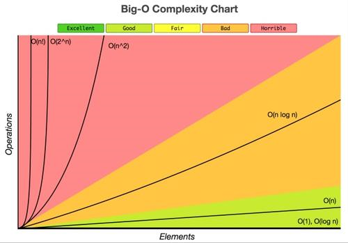
The image is from [xiaoxue.tuxi.com.cn], but this site has been compromised, so please do not visit.

Regarding logarithmic complexity, here’s an example for better understanding:

int count = 1;
while(count < n)
    count = count * 2;

If ( n = ? ), what are the execution counts?

n    counts
2    1
4    2
8    3
... ...

It can be observed that ( n = 2^{(counts)} ). As ( n ) approaches infinity, let’s denote counts as ( m ) on the coordinate axes, then:

According to the concept of logarithm, we can determine ( m = \log_2 n ).

In simple terms, if calculations exhibit such variations in scenario, you can derive a function formula or create a table, substitute some simple numbers, identify patterns, and then express it using mathematical notation.