A Comprehensive Guide to Implementing a KV Database Using LSM Tree Principles

[TOC]

A while ago, I came across the concept of LSM Tree while studying data structures, which prompted me to attempt building a simple KV database based on the design principles of LSM Tree.

The code has been open-sourced, and the repository can be found at: https://github.com/whuanle/lsm

I chose to implement the LSM Tree database using the Go language. The implementation of the LSM Tree involves handling file read/write operations, locking mechanisms, data lookup, file compression, and more, which has enhanced my experience with Go coding. The project also makes use of some basic algorithms like stacks and binary search trees, which helps reinforce foundational algorithm skills. Setting appropriate challenges for oneself can elevate technical abilities.

Next, let’s explore the design philosophy behind LSM Tree and how to implement a KV database.

Design Philosophy

What is LSM Tree?

The full name of LSM Tree is Log-Structured Merge Tree, a data structure for key-value type databases. As far as I know, NoSQL databases like Cassandra and ScyllaDB utilize LSM Tree.

The core theory behind LSM Tree is that sequential disk writes are significantly faster than random writes. Since disk I/O is the largest factor affecting read/write performance in any database, organizing database files effectively and making full use of disk read/write mechanisms can boost database performance. LSM Tree first buffers all write operations in memory. When the memory usage reaches a threshold, the data is flushed to disk. This process involves only sequential writes and avoids random writes, thus LSM excels in write performance.

I will refrain from elaborating on the concept of LSM Tree; interested readers can refer to the materials listed below.

References

"What is a LSM Tree?"

https://dev.to/creativcoder/what-is-a-lsm-tree-3d75

"Understanding LSM Tree: An Efficient Read and Write Storage Engine" by Sheng Bing:

https://mp.weixin.qq.com/s/7kdg7VQMxa4TsYqPfF8Yug

"Implementing LSM Database From Scratch in 500 Lines of Code" by Xiao Hansong:

https://mp.weixin.qq.com/s/kCpV0evSuISET7wGyB9Efg

"Golang Practice on LSM-Related Content" by Xiao Wu Zi Da Xia:

https://blog.csdn.net/qq_33339479

"SM-based Storage Techniques: A Survey" Chinese Translation:

https://zhuanlan.zhihu.com/p/400293980

Overall Structure

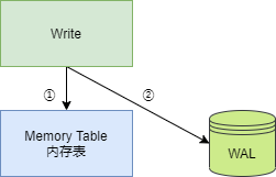
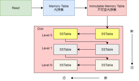
The following diagram illustrates the overall structure of LSM Tree, which can be divided into two main parts: memory and disk files. The disk files consist of database files (SSTable files) and WAL log files.

The memory table is designed to buffer write operations, and whenever a Key/Value is written to the memory table, it is also logged in the WAL file, which can be used as a basis for recovering data in the memory table. When the program starts, it checks for the presence of a WAL file in the directory. If one exists, it will read the WAL file to restore the memory table.

In the disk files, there are multilayer database files, with multiple SSTable files existing within each layer. The database files of the next layer are generated from the compressed merges of the database files from the previous layer, hence, the greater the layer, the larger the database files.

Now, let's delve deeper into the design principles of the different components of LSM Tree and the stages involved in performing read/write operations.

Memory Table

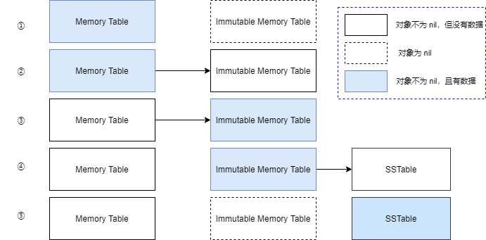
In LSM Tree’s memory space, there are two memory tables: a mutable Memory Table and an immutable Immutable Memory Table; both share the same data structure, typically a binary search tree.

Initially, when the database is empty, the Memory Table is empty, meaning it has no elements, while the Immutable Memory Table is nil, indicating no memory has been allocated yet. At this point, all write operations occur on the Memory Table, including setting the values for Keys and deleting Keys. Upon a successful write to the Memory Table, the operation information is logged in the WAL file.

However, the number of Key/Value pairs stored in the Memory Table cannot become too large, or it may consume excessive memory. Therefore, generally, when the number of Keys in the Memory Table reaches a threshold, the Memory Table becomes an Immutable Memory Table, and a new Memory Table is created. The Immutable Memory Table will be converted into an SSTable at an appropriate time, subsequently stored in the disk files.

Thus, the Immutable Memory Table is a temporary object, only existing temporarily while syncing the elements in memory to the SSTable.

It’s important to note that once the memory table has been synced to the SSTable, the WAL file needs to be deleted. The data that can be recovered using the WAL file should match the current KV elements in memory. This means that the WAL file can restore the last operational state of the program; if the current memory table has already moved to the SSTable, then retaining the WAL file is unnecessary. It should thus be deleted and a new empty WAL file should be created.

There are different implementations regarding the WAL segment; some maintain a single global WAL file, while others may use multiple WAL files, depending on the specific scenario.

WAL

WAL stands for Write Ahead Log. When performing write operations (inserting, modifying, or deleting Keys), since the data is held in memory, it’s crucial to promptly log these write operations into the WAL file to prevent data loss due to program crashes or system failures. Upon the next program startup, the program can read the operation records from the WAL file and restore the state prior to the program’s exit.

The logs retained in the WAL record all operations performed on the current memory table. When restoring the previous memory table from WAL, each operation must be read from the WAL file and reapplied to the memory table, essentially redoing the various write operations. Hence, writing directly to the memory table and recovering data from the WAL both effectively achieve the same result.

It can be said that the WAL logs the operational process, while the binary search tree stores the final results.

The purpose of the WAL is to restore all write operations on the memory table and reapply these operations sequentially to ensure the memory table is returned to its previous state.

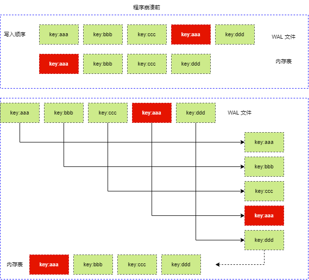
The WAL file is not a binary backup of the memory table; rather, it backup the write operations, and the restoration is based on the write process, not the memory data.

SSTable Structure

SSTable stands for Sorted String Table, which serves as the persistent file for the memory table.

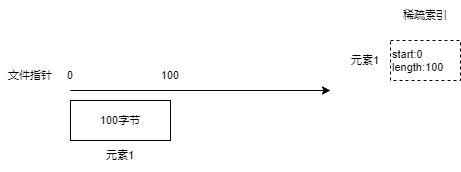
An SSTable file consists of three parts: data area, sparse index area, and metadata, as shown in the following diagram.

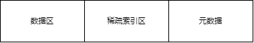
When converting the memory table to SSTable, we first traverse the Immutable Memory Table, sequentially compress each KV pair into binary data, and create a corresponding index structure to record the insertion position and length of this binary KV. All binary KVs are placed at the beginning of the disk file, followed by all the index structures converted to binary format after the data area. Finally, information about the data area and index area is recorded in a metadata structure and written to the end of the file.

Each element in memory has a Key, and when transforming the memory table into SSTable, the elements are sorted by Key and converted into binary to be stored at the beginning of the file, namely in the data area.

But how do we separate each element from the data area?

Different developers might set various structures for SSTable, and the methods for converting memory tables to SSTable might differ as well. Hence, I will only describe my approach while writing the LSM Tree.

My approach was to process each element one at a time when generating the data area instead of handling the entire set of elements as binary at once.

First, a Key/Value element is generated as binary and placed at the beginning of the file, and then an index is constructed to record the starting position and length of this element's binary data in the file. This index is temporarily stored in memory.

Next, the remaining elements are processed continuously while generating corresponding indexes in memory.

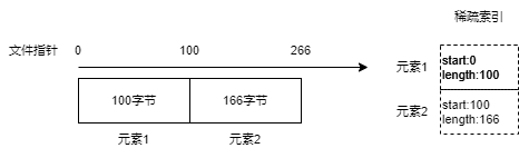
The sparse index denotes the data block of each index executed in the file.

Once all elements are processed, the SSTable file’s data area has been created. Following this, all index collections must be generated as binary data and appended to the file.

Finally, we also need to create metadata for the starting positions and lengths of the data area and sparse index area to enable subsequent reading and splitting of the data area and sparse index area into distinct processing.

The structure of the metadata is simple, comprising four values:

// Data area starting index
dataStart int64
// Data area length
dataLen int64
// Sparse index area starting index
indexStart int64
// Sparse index area length
indexLen int64

The metadata is appended to the end of the file and has a fixed byte length.

When reading an SSTable file, we first read the last few bytes of the file, such as 64 bytes, then restore field values based on every 8 bytes to generate the metadata, allowing us to subsequently handle the data area and sparse index area.

SSTable Elements and Index Structure

To store a Key/Value in the data area, the file block containing this Key/Value element is referred to as a block. To represent Key/Value, we can define such a structure:

Key 
Value
Deleted

Then, we convert this structure into binary data and write it into the data area of the file.

To locate the position of the Key/Value in the data area, we also need to define an index, structured as follows:

Key
Start
Length

Each Key/Value utilizes an index for localization.

SSTable Tree

Each time the memory table transforms into SSTable, an SSTable file is created; hence, we need to manage these SSTable files to prevent an excessive number of files.

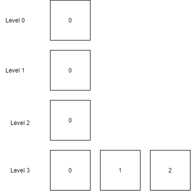
The following illustrates the organizational structure of SSTable files in LSM Tree.

In the above diagram, we can see that the database comprises numerous SSTable files, which are segregated into different layers. To manage the SSTable across different layers, a tree structure organizes all SSTable files on disk, allowing management of the size of different layers or the number of SSTables.

Regarding the SSTable Tree, three key points should be noted:

1. The SSTable files in layer 0 are all converted from the memory table.

2. Except for layer 0, SSTable files in the next layer can only be generated by compressing and merging SSTable files from the previous layer. SSTable files in one layer may merge into a new SSTable for the next layer only when the total file size or count reaches a threshold.

3. Each layer of SSTable has a sequence based on the generation timestamp. This feature is useful for locating data across all SSTables.

Given that each time the memory table is persisted, a new SSTable file is created, the number of SSTable files will increase. As the number of files grows, it requires more file handles and slows down data retrieval across multiple files. If not controlled, excessive files can result in degraded read performance and inflated space usage—a phenomenon known as space amplification and read amplification.

Since SSTables are immutable, modifying a Key or deleting a Key can only be marked in a new SSTable, not altered; this can result in multiple SSTables containing the same Key, making the files bloated.

Therefore, it is also necessary to compress and merge small SSTable files into a larger SSTable file for storage in the next layer to enhance read performance.

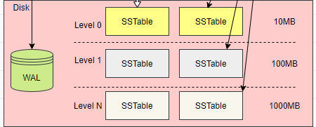
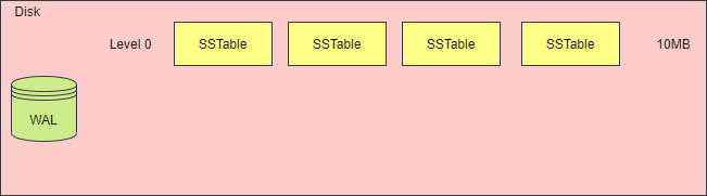
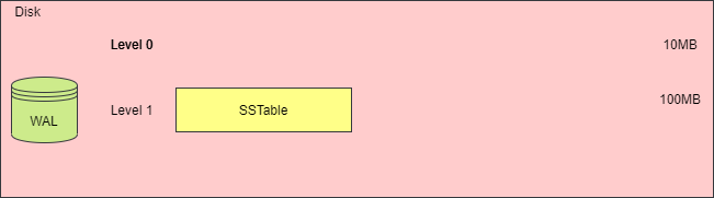
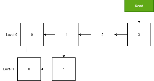
When the total size of SSTable files in one layer exceeds a threshold or when the number of SSTable files is too high, a merge action must be triggered to generate a new SSTable file, place it in the next layer, and remove the old SSTable files. The following diagrams illustrate this process.

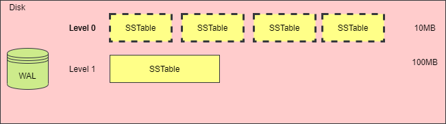
While merging and compressing SSTables can mitigate space amplification and read amplification issues, the process of merging several SSTables into one requires loading each SSTable file, reading its content into memory, creating a new SSTable file, and deleting the old files, which can consume substantial CPU time and disk I/O. This phenomenon is referred to as write amplification.

The diagram below illustrates the changes in storage space before and after merging.

In-Memory SSTable

When the program starts, it will load the metadata and sparse index area of each SSTable into memory, essentially caching the list of Keys from SSTable. When searching for a Key in the SSTable, it first checks the sparse index area in memory. If a Key is found, the associated binary data of the Key/Value will be read from the disk file based on the index’s Start and Length, then converted from binary to the Key/Value structure.

Thus, to determine whether an SSTable contains a certain Key, a lookup is performed in memory, a process that is quite fast. The actual reading from the file occurs only when the value of a Key is needed.

However, when the number of Keys becomes overly large, caching them all in memory can consume a significant amount of memory, and searching through them individually can also take time. To expedite the check for a Key’s existence, a Bloom Filter can be employed.

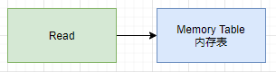
Data Lookup Process

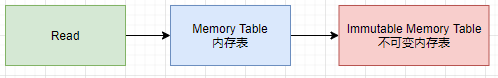
To start, we query the Key from the Memory Table.

If the Key isn’t found in the Memory Table, we then search within the Immutable Memory Table.

In my implementation of the LSM Tree database, there exists only a Memory Table, with no Immutable Memory Table.

If the Key is still not located in either memory table, the search proceeds to the SSTable list.

We begin by querying the SSTable table in layer 0, starting from the most recent SSTable. If the Key is not found, we check other SSTables in the same layer. If it’s still not found, we then move to the next layer.

When the Key is eventually located, regardless of its status (valid or deleted), we stop the search and return the value of this Key, along with the deletion flag.

Implementation Process

In this section, I will outline the general thoughts for implementing LSM Tree and provide some code examples. However, for the complete code, please refer to the repository; here I will only present the definitions relevant to the implementation without going into specific code details.

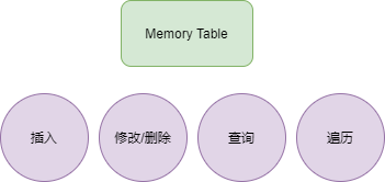
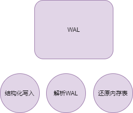
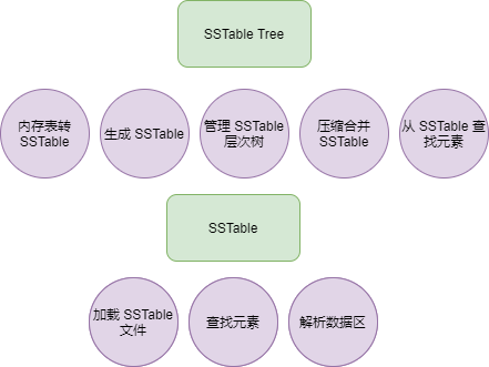
The following diagram shows the primary focus areas of the LSM Tree:

For the memory table, we need to implement CRUD operations and traversal.

For the WAL, it’s necessary to log operations to a file and be able to recover the memory table from the WAL file.

Regarding SSTable, functionality must exist to load file information and search for corresponding data.

The SSTable Tree is responsible for managing all SSTables and handling file merges, etc.

Representation of Key/Value

As a Key/Value database, it must be capable of storing values of any type. Although Go 1.18 introduced generics, generic structs do not offer the flexibility needed to store arbitrary values. To solve the problem of storing various types of Values, I opted not to use generic structs. The type and meaning of the stored data are not crucial for the database itself; this is relevant only to the end-user. Therefore, I can directly convert the value to a binary format for storage and convert it back to its corresponding type when retrieving data.

Define a structure to hold any type of value:

// Value represents a KV
type Value struct {
	Key     string
	Value   []byte
	Deleted bool
}

The reference path for the Value struct is kv.Value.

For example, with a struct like this:

type TestValue struct {
	A int64
	B int64
	C int64
	D string
}

We can serialize it to binary and store it in the Value field.

data,_ := json.Marshal(value)

v := Value{
    Key: "test",
    Value: data,
    Deleted: false,
}

The Key/Value pair is serialized with JSON, converted into binary, and stored in-memory.

This means that in the LSM Tree, even if a Key is deleted, the actual element isn’t removed; it’s just marked as deleted. Therefore, to ascertain the search results, we must define an enumeration to determine whether the found Key is valid.

// SearchResult indicates the search outcome
type SearchResult int

const (
	// None indicates not found
	None SearchResult = iota
	// Deleted indicates it has been deleted 
	Deleted
	// Success indicates found successfully
	Success
)

For code related aspects, readers can refer to: https://github.com/whuanle/lsm/blob/1.0/kv/Value.go

Implementation of Memory Table

In the LSM Tree, the memory table is a binary search tree. Operations on this binary search tree primarily include setting values, inserting, searching, and traversal. Detailed code can be found here:

https://github.com/whuanle/lsm/blob/1.0/sortTree/SortTree.go

Now let’s briefly explain the implementation of the binary search tree.

Assuming the list of Keys to be inserted is [30,45,25,23,17,24,26,28], the structure of the memory table after insertion is as follows:

In developing the binary search tree, I encountered several areas prone to error, so here are some common pitfalls to avoid.

首先，我们要记住：After the node is inserted, its position will not change, it cannot be removed, nor can it be swapped.

The first point, Newly inserted nodes can only be leaf nodes.

Here is a correct insertion operation:

As shown in the figure, with nodes 23, 17, and 24 already existing, inserting 18 requires placing it as the right child of 17.

Below is an incorrect insertion operation:

During the insertion operation, the position of the old nodes cannot be moved, nor can the relationship between left and right children be changed.

The second point, When deleting a node, it can only be marked as deleted and cannot actually be removed.

Definition of Binary Search Tree Structure

The structure and method definitions of the binary search tree are as follows:

// treeNode ordered tree node
type treeNode struct {
	KV    kv.Value
	Left  *treeNode
	Right *treeNode
}

// Tree ordered tree
type Tree struct {
	root   *treeNode
	count  int
	rWLock *sync.RWMutex
}


// Search searches for the value of a key
func (tree *Tree) Search(key string) (kv.Value, kv.SearchResult) {
}

// Set sets the value of a key and returns the old value
func (tree *Tree) Set(key string, value []byte) (oldValue kv.Value, hasOld bool) {
}

// Delete deletes a key and returns the old value
func (tree *Tree) Delete(key string) (oldValue kv.Value, hasOld bool) {
}

For specific code implementations, please refer to: https://github.com/whuanle/lsm/blob/1.0/sortTree/SortTree.go

Since Go's string type is a value type, it can be compared directly, which simplifies much of the code when inserting Key/BValue.

Insertion Operation

Since the tree is ordered, when inserting Key/Value, comparisons are made from top to bottom at the root node based on the size of Key, and it is inserted as a leaf node in the tree.

The insertion process can be divided into various cases.

The first case: When the relevant Key does not exist, it is directly inserted as a leaf node, as either the left child or the right child of the previous layer element.

		if key < current.KV.Key {
			// Left child is empty, insert to the left
			if current.Left == nil {
				current.Left = newNode
                // ... ...
			}
			// Continue comparing to the next layer
			current = current.Left
		} else {
			// Right child is empty, insert to the right
			if current.Right == nil {
				current.Right = newNode
                // ... ...
            }
			current = current.Right
        }

The second case: When the Key already exists, this node may be valid, and we only need to replace the Value; this node may have been marked for deletion, in which case we need to replace the Value and change the Deleted flag to false.

			node.KV.Value = value
			isDeleted := node.KV.Deleted
			node.KV.Deleted = false

So, how is the time complexity when inserting a Key/Value into the binary search tree?

If the binary search tree is relatively balanced, meaning left and right are symmetric, the time complexity for insertion operations is O(logn).

As shown in the following diagram, if there are 7 nodes in the tree, only three layers exist, thus at most three comparisons are needed during insertion.

If the binary search tree is unbalanced, the worst-case scenario is that all nodes are on either the left side or the right side, which leads to a time complexity of O(n) for insertion operations.

As shown in the following diagram, if there are four nodes in the tree, there are four layers, meaning at most four comparisons are needed during insertion.

For the insertion node code, please refer to: https://github.com/whuanle/lsm/blob/5ea4f45925656131591fc9e1aa6c3678aca2a72b/sortTree/SortTree.go#L64

Lookup

When searching for a Key in a binary search tree, based on the size of the Key, choose to either continue with the left child or the right child for the next layer of search. Below is the example of search code:

	currentNode := tree.root
	// Ordered search
	for currentNode != nil {
		if key == currentNode.KV.Key {
			if currentNode.KV.Deleted == false {
				return currentNode.KV, kv.Success
			} else {
				return kv.Value{}, kv.Deleted
			}
		}
		if key < currentNode.KV.Key {
			// Continue comparing to the next layer
			currentNode = currentNode.Left
		} else {
			// Continue comparing to the next layer
			currentNode = currentNode.Right
		}
	}

Its time complexity is consistent with that of insertion.

For the lookup code, please refer to: https://github.com/whuanle/lsm/blob/5ea4f45925656131591fc9e1aa6c3678aca2a72b/sortTree/SortTree.go#L34

Deletion

During deletion, you only need to find the corresponding node, clear its Value, and set the delete flag; the node itself cannot be deleted.

				currentNode.KV.Value = nil
				currentNode.KV.Deleted = true

Its time complexity is consistent with that of insertion.

For the deletion code, please refer to: https://github.com/whuanle/lsm/blob/5ea4f45925656131591fc9e1aa6c3678aca2a72b/sortTree/SortTree.go#L125

Traversal Algorithm

Reference code: https://github.com/whuanle/lsm/blob/5ea4f45925656131591fc9e1aa6c3678aca2a72b/sortTree/SortTree.go#L175

To traverse the nodes of the binary search tree in order, a recursive algorithm is the simplest approach; however, when the tree has high levels, recursion can consume a lot of memory space. Therefore, we need to use a stack algorithm to traverse the tree and systematically retrieve all nodes.

In Go, a slice is used to implement the stack: https://github.com/whuanle/lsm/blob/1.0.0/sortTree/Stack.go

The in-order traversal of the binary search tree is essentially pre-order traversal. After completing the traversal, the obtained set of nodes will have their Key in order.

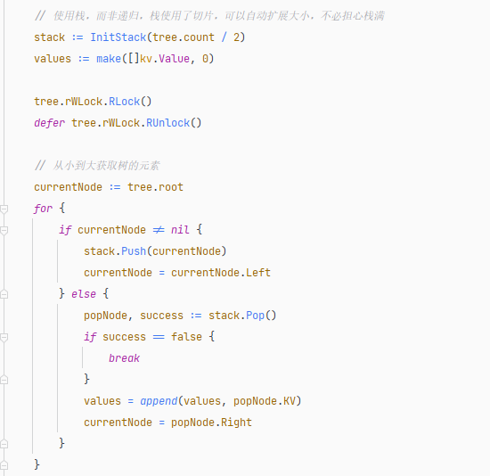
The reference code is as follows:

	// Using the stack instead of recursion, the stack can expand automatically
	stack := InitStack(tree.count / 2)
	values := make([]kv.Value, 0)

	tree.rWLock.RLock()
	defer tree.rWLock.RUnlock()

	// Get tree elements in ascending order
	currentNode := tree.root
	for {
		if currentNode != nil {
			stack.Push(currentNode)
			currentNode = currentNode.Left
		} else {
			popNode, success := stack.Pop()
			if success == false {
				break
			}
			values = append(values, popNode.KV)
			currentNode = popNode.Right
		}
	}

Traversal code: https://github.com/whuanle/lsm/blob/33d61a058d79645c7b20fd41f500f2a47bc95357/sortTree/SortTree.go#L175

The stack size is initially allocated to half the number of tree nodes, which is appropriate if the tree is balanced. Also, not all nodes need to be pushed onto the stack before retrieval; elements can be retrieved from the stack as soon as there are no left children.

If the tree is unbalanced, the actual stack space may indeed be larger; however, this stack uses slices, and if stack space is insufficient, it will expand automatically.

The traversal process is shown in the animated diagram below:

Creating the animation is difficult~

It can be observed that the required stack space relates to the height of the binary tree.

WAL

The structure of WAL is defined as follows:

type Wal struct {
	f    *os.File
	path string
	lock sync.Locker
}

WAL needs to possess two capabilities:

1. When the program starts, it should be able to read the contents of the WAL file and restore it to an in-memory table (binary search tree).
2. After the program starts, insert and delete operations on the in-memory table must be recorded in the WAL file.

Reference code: https://github.com/whuanle/lsm/blob/1.0/wal/Wal.go

Next, let's explain the author's WAL implementation process.

Below is a simplified code for writing to the WAL file:

// Record log
func (w *Wal) Write(value kv.Value) {
	data, _ := json.Marshal(value)
	err := binary.Write(w.f, binary.LittleEndian, int64(len(data)))
	err = binary.Write(w.f, binary.LittleEndian, data)
}

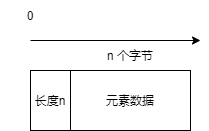
As you can see, it first writes an 8-byte value, followed by the serialized Key/Value.

In order to properly restore data from the WAL file when the program starts, it is essential to have a clear separation in the WAL file so that each element operation can be correctly read.

Therefore, each element written to the WAL must record its length, represented using the int64 type, which occupies 8 bytes.

WAL File Recovery Process

In the previous section, an element written to the WAL file consists of the element data and its length. Thus, the WAL file structure can be thought of as follows:

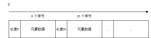
Therefore, when using the WAL file to recover data, the first step is to read the first 8 bytes from the file to determine the byte count n of the first element. Then, load the binary data in the range 8 ~ (8+n) into memory and deserialize it to kv.Value type using json.Unmarshal().

Next, read the 8 bytes located at (8+n) ~ (8+n)+8 to determine the data length of the next element, and continue this process until the entire WAL file is read.

Generally, the WAL file will not be very large. Thus, during program startup, the data recovery process can load the entire WAL file into memory and then read and deserialize each element one by one, identifying whether the operation is a Set or Delete, then calling the corresponding Set or Delete methods of the binary search tree to add elements to the nodes.

Reference code is as follows:

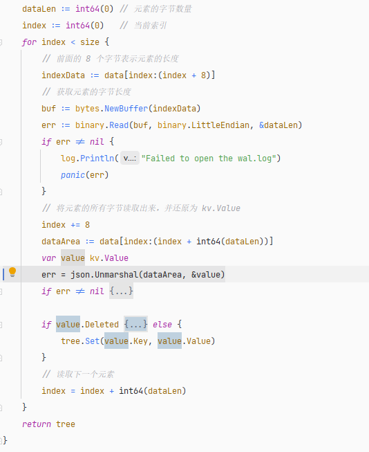
Code location: https://github.com/whuanle/lsm/blob/4faddf84b63e2567118f0b34b5d570d1f9b7a18b/wal/Wal.go#L43

SSTable and SSTable Tree

The code related to SSTable is relatively extensive, and it can be divided into three parts: saving SSTable files, parsing SSTable from files, and searching for Keys.

The list of all SSTable code files written by the author is as follows:

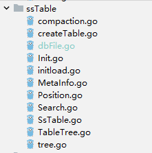
SSTable Structure

The structure of the SSTable is defined as follows:

// SSTable table, stored in disk files
type SSTable struct {
	// File handle
	f        *os.File
	filePath string
	// Metadata
	tableMetaInfo MetaInfo
	// Sparse index list of the file
	sparseIndex map[string]Position
	// Sorted key list
	sortIndex []string
	lock sync.Locker
}

The elements in sortIndex are ordered, and the memory locations for the elements are contiguous, which helps with CPU cache efficiency and improves lookup performance. Additionally, a bloom filter can be used to quickly determine if this Key exists in the SSTable.

Once the relevant SSTable is confirmed, the index can be looked up in sparseIndex to locate the element in the file.

The definitions for metadata and sparse index structures are as follows:

type MetaInfo struct {
	// Version number
	version int64
	// Starting index of the data area
	dataStart int64
	// Length of the data area
	dataLen int64
	// Starting index of the sparse index area
	indexStart int64
	// Length of the sparse index area
	indexLen int64
}

// Position element positioning, stored in the sparse index area, indicating the starting position and length of an element
type Position struct {
	// Starting index
	Start int64
	// Length
	Len int64
	// Key has been deleted
	Deleted bool
}

It can be seen that a SSTable structure needs to point not only to the disk file but also to cache certain data in memory. However, different developers may handle this differently. For example, the author has fixed this pattern from the start and decided to cache the Keys list in memory while using a dictionary to cache element positions.

	// Sparse index list of the file
	sparseIndex map[string]Position
	// Sorted key list
	sortIndex []string

In reality, only keeping the sparseIndex map[string]Position can also accomplish all lookup operations. The sortIndex []string is not strictly necessary.

SSTable File Structure

SSTable files are divided into three parts: the data area, the sparse index area, and the metadata/file index. The content stored is related to the data structure defined by the developer. As illustrated below:

The data area contains a list of serialized Value structures, while the sparse index area consists of serialized Position lists. However, the serialization processing methods of the two areas are different.

The sparse index area is serialized as a map[string]Position, allowing for direct deserialization of the sparse index area back to the map[string]Position type when reading the file.

The data area, by contrast, is made up of serialized kv.Value appended sequentially. Therefore, it cannot be entirely deserialized to []kv.Value; each block in the data area must be progressively read via Position and then deserialized to kv.Value.

SSTable Tree Structure and Managing SSTable Files

To organize a large number of SSTable files, we also need a struct to manage all disk files in a hierarchical manner.

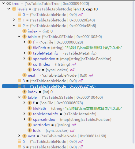
We need to define a TableTree structure, defined as follows:

// TableTree tree
type TableTree struct {
	levels []*tableNode  // This part is a linked list array
	// Prevent conflicts when inserting, compressing, or deleting SSTables
	lock *sync.RWMutex
}

// Linked list representing each layer of SSTable
type tableNode struct {
	index int
	table *SSTable
	next  *tableNode
}

To facilitate layering SSTables and marking the order of their insertion, a naming convention for SSTable files must be established.

如上文件所示：

├── 0.0.db
├── 1.0.db
├── 2.0.db
├── 3.0.db
├── 3.1.db
├── 3.2.db

SSTable files are composed of {level}.{index}.db, where the first number represents the level of the SSTable, and the second number indicates the index within that level.

Here, a larger index indicates that the file is newer.

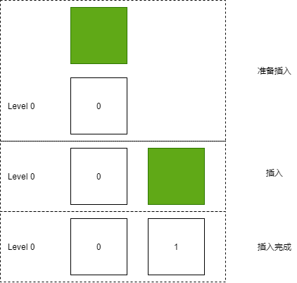
Inserting SSTable Files

When converting from the memtable to SSTable, each SSTable being converted is appended at the end of Level 0.

Each layer's SSTable is managed using a linked list:

type tableNode struct {
	index int
	table *SSTable
	next  *tableNode
}

Therefore, during the insertion of SSTable, we traverse downward and place it at the end of the linked list.

The code snippet for inserting nodes into the linked list is as follows:

		for node != nil {
			if node.next == nil {
				newNode.index = node.index + 1
				node.next = newNode
				break
			} else {
				node = node.next
			}
		}

The conversion from memtable to SSTable involves several operations. Readers are encouraged to refer to the code: https://github.com/whuanle/lsm/blob/1.0/ssTable/createTable.go

Reading SSTable Files

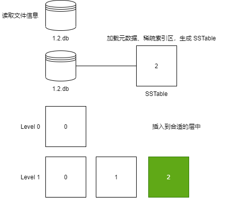
When the program starts, it needs to read all SSTable files in the directory into the TableTree, and then load the sparse index regions and metadata of each SSTable.

The author's LSM Tree processing is illustrated in the following diagrams:

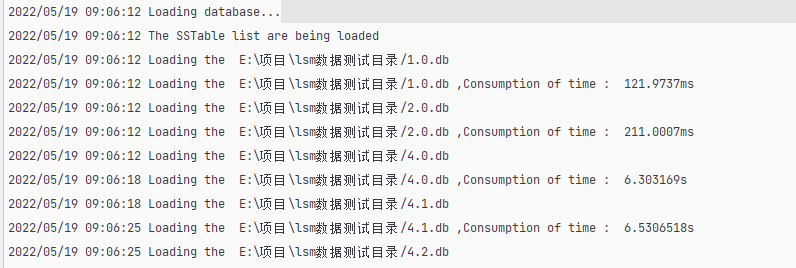
The time taken by the author's LSM Tree to load these files was 19.4259983 seconds.

The code for the loading process can be found here: https://github.com/whuanle/lsm/blob/1.0/ssTable/Init.go

Let's discuss the general loading process.

First, read all .db files in the directory:

	infos, err := ioutil.ReadDir(dir)
	if err != nil {
		log.Println("Failed to read the database file")
		panic(err)
	}
	for _, info := range infos {
		// If it is an SSTable file
		if path.Ext(info.Name()) == ".db" {
			tree.loadDbFile(path.Join(dir, info.Name()))
		}
	}

Then create an SSTable object and load the file's metadata and sparse index area:

	// Load file handle and table metadata simultaneously
	table.loadMetaInfo()
    // Load the sparse index area
	table.loadSparseIndex()

Finally, insert into the designated position in TableTree according to the name of the .db file:

Merging SSTable Files

When there are too many SSTable files in a layer or the files are too large, it is necessary to merge the SSTable files in that layer to create a new SSTable that does not contain duplicate elements and place it into a new layer.

Therefore, the author's approach is to use a new thread after the program starts to check if the memtable needs to be converted into SSTable or if the SSTable layer needs to be compacted. The checks start from Level 0 and examine two condition thresholds: the first is the number of SSTables, and the second is the total size of the SSTable files in that layer.

The merging threshold for SSTable files must be set at program startup.

	lsm.Start(config.Config{
		DataDir:    `E:\Project\lsm_data_test_directory`,
		Level0Size: 1,		// Threshold for the total size of all SSTable files in level 0
		PartSize:   4,		// Threshold for the number of SSTables in each layer
		Threshold:  500,    // Memtable element threshold
        CheckInterval: 3, // Compaction time interval
	})

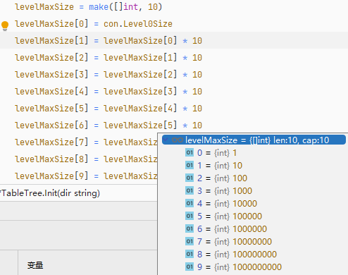
The total size of all SSTable files in each layer is based on the generation of Level 0. For example, when you set Level 0 to 1MB, Level 1 will be 10MB, and Level 2 will be 100MB. Users only need to set the total size threshold for Level 0.

Now let's explain the process of merging SSTable files.

The complete code for compaction and merging can be found at: https://github.com/whuanle/lsm/blob/1.0/ssTable/compaction.go

Here is the initial file tree:

First, create a binary search tree object:

	memoryTree := &sortTree.Tree{}

Then, in Level 0, start from the SSTable with the smallest index, read each block in the file data area, deserialize it, and perform insertion or deletion operations.

		for k, position := range table.sparseIndex {
			if position.Deleted == false {
				value, err := kv.Decode(newSlice[position.Start:(position.Start + position.Len)])
				if err != nil {
					log.Fatal(err)
				}
				memoryTree.Set(k, value.Value)
			} else {
				memoryTree.Delete(k)
			}
		}

All SSTables from Level 0 are loaded into the binary search tree to merge all elements.

Then, convert the binary search tree into SSTable and insert it into Level 1.

Next, delete all SSTable files from Level 0.

Note: The author’s compaction method loads files into memory and uses slices to store file data, which may lead to errors due to excessive capacity.

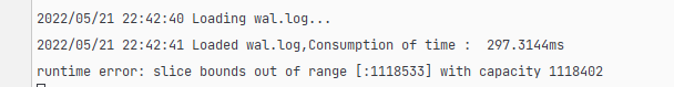
This is a point worth noting.

SSTable Lookup Process

The complete code can be referenced at: https://github.com/whuanle/lsm/blob/1.0/ssTable/Search.go

When looking for an element, we first search in the memtable; if it cannot be found, then we need to search through each SSTable in the TableTree.

	// Iterate through each layer's SSTable
	for _, node := range tree.levels {
		// Organize the SSTable list
		tables := make([]*SSTable, 0)
		for node != nil {
			tables = append(tables, node.table)
			node = node.next
		}
		// Start searching from the last SSTable
		for i := len(tables) - 1; i >= 0; i-- {
			value, searchResult := tables[i].Search(key)
			// If not found, continue to the next SSTable
			if searchResult == kv.None {
				continue
			} else { // If found or marked as deleted, return the result
				return value, searchResult
			}
		}
	}

When searching within an SSTable, binary search is used:

	// Element positioning
	var position Position = Position{
		Start: -1,
	}
	l := 0
	r := len(table.sortIndex) - 1

	// Binary search to check if key exists
	for l <= r {
		mid := int((l + r) / 2)
		if table.sortIndex[mid] == key {
			// Get the element's position
			position = table.sparseIndex[key]
			// If the element has been deleted, return
			if position.Deleted {
				return kv.Value{}, kv.Deleted
			}
			break
		} else if table.sortIndex[mid] < key {
			l = mid + 1
		} else if table.sortIndex[mid] > key {
			r = mid - 1;
		}
	}

	if position.Start == -1 {
		return kv.Value{}, kv.None
	}

That concludes the writing on the LSM Tree database. Next, let’s understand the author's database performance and usage.

Simple Usage Testing

Example code can be found here: https://gist.github.com/whuanle/1068595f46824466227b93ef583499d3

First, download the dependency package:

go get -u github.com/whuanle/lsm@v1.0.0

Then, initialize the database using lsm.Start(), and perform insert, delete, search, and update operations on the Key. Sample code is as follows:

package main

import (
	"fmt"
	"github.com/whuanle/lsm"
	"github.com/whuanle/lsm/config"
)

type TestValue struct {
	A int64
	B int64
	C int64
	D string
}

func main() {
	lsm.Start(config.Config{
		DataDir:    `E:\Project\lsm_data_test_directory`,
		Level0Size: 1,
		PartSize:   4,
		Threshold:  500,
        CheckInterval: 3, // Compaction time interval
	})
	// 64 bytes
	testV := TestValue{
		A: 1,
		B: 1,
		C: 3,
		D: "00000000000000000000000000000000000000",
	}

	lsm.Set("aaa", testV)

	value, success := lsm.Get[TestValue]("aaa")
	if success {
		fmt.Println(value)
	}

	lsm.Delete("aaa")
}

testV is 64 bytes, while kv.Value stores the value of testV, which is 131 bytes.

File Compression Test

We can write a function that creates keys from any 6 letters out of 26 letters and insert them into the database to observe file compression, merging, and insertion speed.

Number of elements inserted at different loop levels:

| 1 | 2 | 3 | 4 | 5 | 6 |
| ---- | ---- | ------ | ------- | ---------- | ----------- |
| 26 | 676 | 17,576 | 456,976 | 11,881,376 | 308,915,776 |

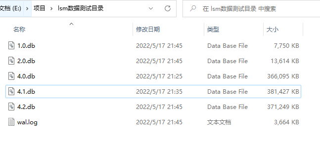
Generated test file list:

The animated process of file compression merging is shown below (about 20 seconds):

Insertion Testing

Here are some informal test results.

Configuration settings when starting the database:

	lsm.Start(config.Config{
		DataDir:    `E:\Project\lsm_data_test_directory`,
		Level0Size: 10,  // Size of SSTable files in Level 0
		PartSize:   4,	 // Number of files per layer
		Threshold:  3000, // Memtable threshold
        CheckInterval: 3, // Compaction time interval
	})
	
	lsm.Start(config.Config{
		DataDir:    `E:\Project\lsm_data_test_directory`,
		Level0Size: 100,
		PartSize:   4,
		Threshold:  20000,
        CheckInterval: 3,
	})

Data insertion:

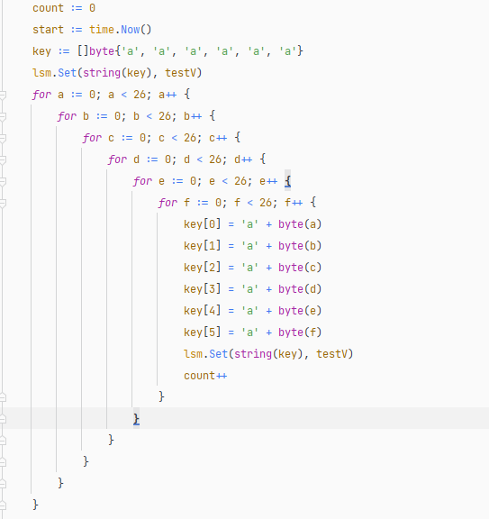
func insert() {

	// 64 bytes
	testV := TestValue{
		A: 1,
		B: 1,
		C: 3,
		D: "00000000000000000000000000000000000000",
	}

	count := 0
	start := time.Now()
	key := []byte{'a', 'a', 'a', 'a', 'a', 'a'}
	lsm.Set(string(key), testV)
	for a := 0; a < 1; a++ {
		for b := 0; b < 1; b++ {
			for c := 0; c < 26; c++ {
				for d := 0; d < 26; d++ {
					for e := 0; e < 26; e++ {
						for f := 0; f < 26; f++ {
							key[0] = 'a' + byte(a)
							key[1] = 'a' + byte(b)
							key[2] = 'a' + byte(c)
							key[3] = 'a' + byte(d)
							key[4] = 'a' + byte(e)
							key[5] = 'a' + byte(f)
							lsm.Set(string(key), testV)
							count++
						}
					}
				}
			}
		}
	}
	elapse := time.Since(start)
	fmt.Println("Insertion complete, data amount:", count, ", time consumed:", elapse)
}

In both tests, the total size of the generated SSTable files was approximately 82MB.

Time consumed during both tests:

Insertion complete, data amount: 456976 , time consumed: 1m43.4541747s

Insertion complete, data amount: 456976 , time consumed: 1m42.7098146s

Thus, each element is 131 bytes, and this database can insert around 4500 records per second in 100 seconds, totaling about 450,000 records.

If the value of kv.Value is relatively large and tested at 3231 bytes, inserting 456976 pieces of data resulted in files of about 1.5GB, consuming 2m10.8385817s, equating to about 3500 records per second.

For inserting larger values of kv.Value, see the code example: https://gist.github.com/whuanle/77e756801bbeb27b664d94df8384b2f9

Load Test

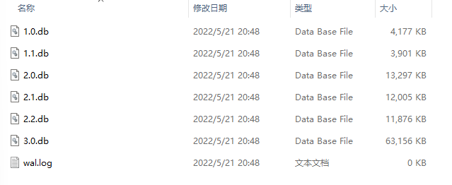
Below is the SSTable file list after inserting 450,000 data records with each element being 3231 bytes. Upon program startup, we need to load these files...

2022/05/21 21:59:30 Loading wal.log...
2022/05/21 21:59:32 Loaded wal.log, Consumption of time :  1.8237905s
2022/05/21 21:59:32 Loading database...
2022/05/21 21:59:32 The SSTable list are being loaded
2022/05/21 21:59:32 Loading the  E:\项目\lsm数据测试目录/1.0.db
2022/05/21 21:59:32 Loading the  E:\项目\lsm数据测试目录/1.0.db , Consumption of time :  92.9994ms
2022/05/21 21:59:32 Loading the  E:\项目\lsm数据测试目录/1.1.db
2022/05/21 21:59:32 Loading the  E:\项目\lsm数据测试目录/1.1.db , Consumption of time :  65.9812ms
2022/05/21 21:59:32 Loading the  E:\项目\lsm数据测试目录/2.0.db
2022/05/21 21:59:32 Loading the  E:\项目\lsm数据测试目录/2.0.db , Consumption of time :  331.6327ms
2022/05/21 21:59:32 The SSTable list are being loaded, consumption of time :  490.6133ms

It can be seen that, except for WAL loading which takes a lot of time (because it needs to be inserted into memory one by one), the loading of SSTable files is relatively fast.

Lookup Testing

When all elements are in memory, even with 450,000 entries, the lookup speed is still very fast. For example, looking up the data for aaaaaa (the minimum Key) and aazzzz (the maximum Key) takes very little time.

The following uses a database file of 3 KB per entry for testing.

Lookup code:

    start := time.Now()
    elapse := time.Since(start)
    v, _ := lsm.Get[TestValue]("aaaaaa") // or aazzzz
    fmt.Println("查找完成，消耗时间：", elapse)
    fmt.Println(v)

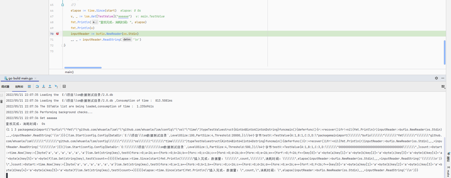
When looking up in the SSTable, the key aaaaaa was written in first, so it will definitely be at the end of the lowest-level SSTable file, which requires more time to access.

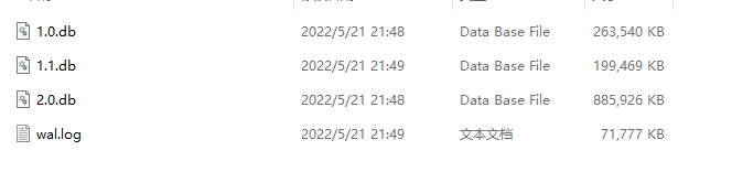
SSTable file list:

├── 1.0.db      116MB
├── 2.0.db		643MB
├── 2.1.db		707MB

About 1.5GB

The key aaaaaa is in 2.0.db, and during the lookup, it will load in the order of 1.0.db, 2.1.db, 2.0.db.

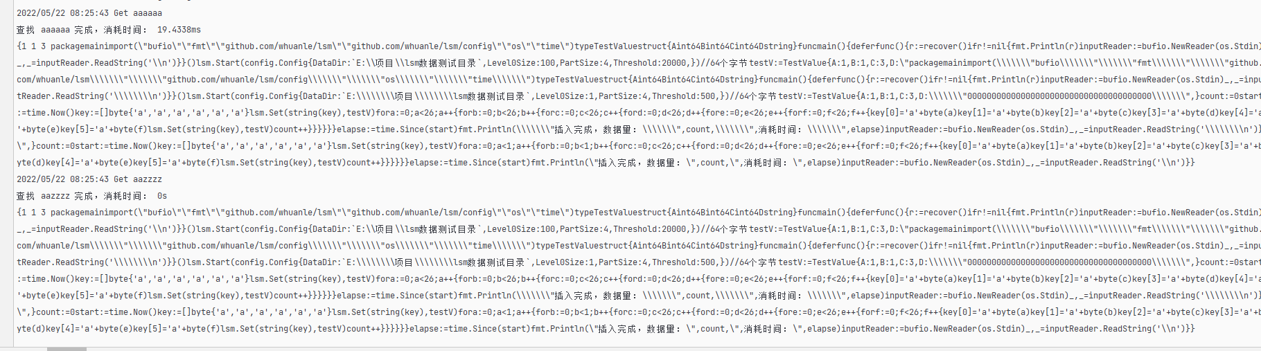
Query speed test:

2022/05/22 08:25:43 Get aaaaaa
查找 aaaaaa 完成，消耗时间： 19.4338ms

2022/05/22 08:25:43 Get aazzzz
查找 aazzzz 完成，消耗时间： 0s

This concludes the introduction to the author's LSM Tree database. For detailed implementation code, please refer to the GitHub repository.