NumPy

NumPy is the fundamental package for scientific computing in Python. It is a Python library that provides a multidimensional array object, various derived objects (like masked arrays and matrices), and a suite of routines for fast operations on arrays, including mathematical operations, logical operations, shape manipulations, sorting, selection, I/O, discrete Fourier transforms, basic linear algebra, basic statistical operations, random simulations, and more.

Official documentation: https://numpy.org/

Simply learning NumPy can be dull because it is geared towards scientific computing. Just learning the various API usages can feel frustrating, as it seems disconnected from artificial intelligence.

Installing numpy is quite straightforward; you can install it directly using the command:

pip install numpy

To test if the installation was successful, run:

import numpy as np
print(np.__version__)

Basic Usage

Basic Data Types

The following table lists common basic types in NumPy.

| Name | Description |
| --- | --- |
| bool_ | Boolean data type (True or False) |
| int_ | Default integer type (similar to long in C, int32 or int64) |
| intc | Same as C's int type, generally int32 or int64 |
| intp | Integer type used for indexing (similar to C's ssize_t, usually int32 or int64) |
| int8 | Byte (-128 to 127) |
| int16 | Integer (-32768 to 32767) |
| int32 | Integer (-2147483648 to 2147483647) |
| int64 | Integer (-9223372036854775808 to 9223372036854775807) |
| uint8 | Unsigned integer (0 to 255) |
| uint16 | Unsigned integer (0 to 65535) |
| uint32 | Unsigned integer (0 to 4294967295) |
| uint64 | Unsigned integer (0 to 18446744073709551615) |
| float_ | Abbreviation for float64 type |
| float16 | Half-precision floating point, consisting of: 1 sign bit, 5 exponent bits, 10 fraction bits |
| float32 | Single-precision floating point, consisting of: 1 sign bit, 8 exponent bits, 23 fraction bits |
| float64 | Double-precision floating point, consisting of: 1 sign bit, 11 exponent bits, 52 fraction bits |
| complex_ | Abbreviation for complex128 type, i.e. 128-bit complex number |
| complex64 | Complex number representing two 32-bit floats (real and imaginary parts) |
| complex128 | Complex number representing two 64-bit floats (real and imaginary parts) |

Each built-in type has a unique character code defining it, as shown below:

| Character | Corresponding Type |
| ---- | ------------------------- |
| b | Boolean |
| i | (signed) integer |
| u | Unsigned integer |
| f | Floating point |
| c | Complex floating point |
| m | timedelta (time interval) |
| M | datetime (date, time) |
| O | (Python) object |
| S, a | (byte-)string |
| U | Unicode |
| V | Raw data (void) |

NumPy has a dtype function used to define variable types, defined as follows:

class numpy.dtype(dtype, align=False, copy=False[, metadata])

For example, this code defines a variable of type int32 in NumPy:

import numpy as np
a = np.dtype(dtype="int32")
print(a)

You can also use a shorthand code:

import numpy as np
a = np.dtype("i")
print(a)

Equivalent code:

import numpy as np
a = np.dtype(np.int32)
print(a)

Running any of these codes will print:

int32

This type is specific to NumPy, not a Python type, so be careful to distinguish. The numeric types in NumPy are actually instances of dtype objects and correspond to unique characters, including np.bool_, np.int32, np.float32, etc.

Since Python is weakly typed, there is no syntax like int32 a = ..., so to clearly define what type this variable should be, you need to use the string name of the type.

You can set this aside for now; it will be used frequently in various contexts with dtype, and you'll get accustomed to it.

It's important to note that np.dtype creates a type identifier but does not itself store variable values.

Example:

import numpy as np

def test(object, dtype):
    if dtype == np.int32:
        print(f"{object} int32")

    elif dtype == np.int64:
        print(f"{object} int64")

    elif dtype == np.str_:
        print(f"{object} str_")

a = 111
b = np.dtype(dtype="int32")
test(a, b)

c = '111'
d = np.dtype(dtype="str")
test(c, d)

Creating Basic Arrays

Numpy provides a multidimensional array object and various derived objects (like masked arrays and matrices), and the most important objects in NumPy are arrays and matrices. Therefore, the most fundamental learning aspect of NumPy is knowing how to work with NumPy arrays.

The procedure for creating arrays in NumPy is defined as follows:

numpy.array(object, dtype=None, copy=True, order=None, subok=False, ndmin=0)

Parameter descriptions:

| Name | Description |
| --- | --- |
| object | Array or nested sequence |
| dtype | Data type of array elements, optional |
| copy | Whether to copy the object, optional |
| order | Array creation style, C for row-major, F for column-major, A for any (default) |
| subok | By default, returns an array that is consistent with the base class type |
| ndmin | Specifies the minimum number of dimensions the generated array should have |

Creating a basic array:

import numpy as np
a = np.array([1, 2, 3])

Creating a multidimensional array:

import numpy as np
a = np.array([[1,  2],  [3,  4]])
print(a)

Defining an array and then generating multidimensional arrays:

import numpy as np
a = np.array([1, 2, 3, 4, 5], ndmin=2)
# Equivalent to np.array([[1, 2, 3, 4, 5]])
print(a)

b = np.array([1, 2, 3, 4, 5], ndmin=3)
# Equivalent to np.array([[[1, 2, 3, 4, 5]]])
print(b)

c = np.array([[1, 2, 3, 4, 5],[1, 2, 3, 4, 5]], ndmin=3)
# Equivalent to np.array([[[1, 2, 3, 4, 5],[1, 2, 3, 4, 5]]])
print(c)

Array Attributes

Since Python is weakly typed, it can feel confusing when trying to learn and understand details. Thus, we try to obtain some documentation comments for our Python code whenever possible.

For example, in the following code, we define an array:

import numpy as np
a = np.array([[1,  2],  [3,  4]])
print(a)

In NumPy, the array type is ndarray[Any, dtype], and the full documentation is as follows:

a: ndarray[Any, dtype] = np.array([[1,  2],  [3,  4]])

Thus, to master NumPy arrays, one essentially needs to understand ndarray.

Some important properties of ndarray are as follows:

| Property | Description |
| --- | --- |
| ndarray.ndim | Rank, i.e., the number of axes or dimensions |
| ndarray.shape | Dimensions of the array, for matrices, n rows and m columns |
| ndarray.size | Total number of elements in the array, equivalent to n*m in .shape |
| ndarray.dtype | The element type of the ndarray object |
| ndarray.itemsize | Size of each element in the ndarray object, in bytes |
| ndarray.flags | Memory information of the ndarray object |
| ndarray.real | Real part of the elements in the ndarray |
| ndarray.imag | Imaginary part of the elements in the ndarray |
| ndarray.data | Buffer containing the actual array elements; normally not needed because elements can usually be accessed via the array index. |

Returning to the previously mentioned numpy.dtype, in conjunction with numpy.array, the example code is as follows:

import numpy
import numpy as np

a = np.array([1, 2])
print(a.dtype)
print(a)

t = np.dtype(numpy.float64)
b = np.array(object=[1, 2], dtype=t)
print(b.dtype)
print(b)

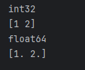
If we do not specify the dtype parameter, then the dtype of the array will be based on the type of the array elements. If dtype is configured, then all array elements will be converted to the corresponding type, such as np.array(object=[1, 2], dtype='float64').

Array Creation

zeros, ones, empty Array Creation

numpy.zeros

numpy.zeros is used to create an array filled with zeros.

Its definition is:

def zeros(shape, dtype=float, order='C', *, like=None, /)

| Parameter | Description |
| --- | --- |
| shape | Shape of the array |
| dtype | Data type, optional |
| order | Has two options "C" and "F" representing row-major and column-major order in which elements are stored in memory. |

Creating an array filled entirely with zeros:

import numpy as np

# Length of 2
a = np.zeros(2)
print(a)

np.zeros() creates arrays of type float64 by default; you can use dtype to customize:

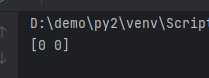
import numpy as np

# Length of 2
a = np.zeros(2, dtype=int)
print(a)

numpy.ones

ones creates an array where all element values are 1.

Its definition is:

def ones(shape, dtype=None, order='C', *, like=None)

Example:

import numpy as np

# Length of 2
a = np.ones(2, dtype=int)
print(a)

Since its API is consistent with numpy.zeros, there's no need to elaborate further.

numpy.empty

Creates an empty array of specified length without initializing the memory area, so the memory allocated might already hold values.

Its definition is:

def empty(shape, dtype=None, order='C', *args, **kwargs)

Example:

import numpy as np

# Length of 2
a = np.empty(2) 
print(a)

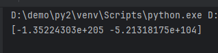
Because it does not initialize memory, the memory area may contain residual data.

Other Notes

Additionally, there are three functions that correspond to prototypical copy functions:

def empty_like(prototype, dtype=None, order=None, subok=None, shape=None)

def zeros_like(prototype, dtype=None, order='K', subok=True, shape=None)

def ones_like(prototype, dtype=None, order='K', subok=True, shape=None)

Their purpose is to create a copy of an identical structure based on the array type, then fill it with corresponding values.

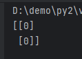
In the example below, a copy of the same structure is made, but filled with the value 0.

import numpy as np

a = np.array([[1],[1]])
b = np.zeros_like(a)
print(b)

Moreover, these three functions can accept tuples to generate multi-dimensional arrays (matrices).

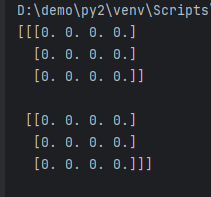
import numpy
import numpy as np

a = np.zeros(shape=(2, 3, 4), dtype=numpy.double)
print(a)

numpy.random

numpy.random is a class, not a function, and it contains several functions for generating random arrays.

Here are some commonly used APIs:

# Generates random samples uniformly distributed in the range [0, 1) of the specified shape.
numpy.random.rand(size)

# Generates random samples from a standard normal distribution (mean = 0, variance = 1). The sample values fall in the range [0, 1).
numpy.random.randn(size)

# Normal distribution with specified mean and variance
numpy.random.normal(loc=0.0, scale=1.0, size=None)

# Generates random values
numpy.random.random(size=None)

# Generates random integers within the given range.
numpy.random.randint(low, high=None, size=None, dtype=int)

# Generates random samples from the specified one-dimensional array.
numpy.random.choice(a, size=None, replace=True, p=None)

# Randomly shuffles the order of the given array.
numpy.random.shuffle(x)

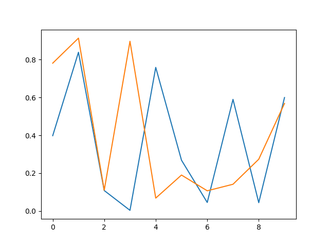
Examples of random number generation and normal distribution generation are as follows:

import numpy as np

a = np.random.rand(10)
b = np.random.rand(10)
print(a)
print(b)

[0.39809428 0.83922059 0.10808865 0.00332159 0.75922001 0.26850704
 0.04497839 0.59012908 0.0438718  0.59988563]
[0.78161896 0.91401858 0.10980276 0.89723959 0.06802148 0.18993732
 0.10664519 0.14121531 0.27353601 0.56878734]

x1 = np.random.randint(10, size=6) # One-dimensional array
x2 = np.random.randint(10, size=(3, 4)) # Two-dimensional array
x3 = np.random.randint(10, size=(3, 4, 5)) # Three-dimensional array

Due to space limitations, further APIs are not elaborated here.

numpy.arange

numpy.arange is used to generate arrays in a regular pattern.

Its definition is as follows:

numpy.arange([start, ]stop, [step, ]dtype=None, *, like=None)

| Parameter | Description |
| --- | --- |
| start | Starting value, default is 0 |
| stop | Ending value (excluding) |
| step | Step size, default is 1 |
| dtype | Data type of the returned ndarray; if not provided, will use the type of the input data. |

numpy.arange defaults to generating an array starting from 0 with an interval of 1.

For example, the following code will generate an array of elements not exceeding 4, i.e., the range is [0, 4).

import numpy as np

# Length of 4
a = np.arange(4)
print(a)

arange(start, stop) specifies the starting and ending ranges, but still with a step size of 1.

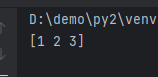
import numpy as np

# Length of 4
a = np.arange(1, 4)
print(a)

arange(start, stop, step) sets custom ranges and step sizes.

import numpy as np


# Length of 4
a = np.arange(1, 10, 3)
print(a)

numpy.linspace

numpy.linspace can generate arrays using linear intervals:

np.linspace(0, 10, num=5)

The meaning of num=5 is to average 5 values between the starting points.

[ 0.  
 2.5 
 5.  
 7.5 
 10. ]

However, the result may not be what we expected, as linspace() includes the starting point, so actually there are 11 numbers from 0-10.

import numpy as np

# Length of 4
a = np.linspace(0, 10, num=10)
print(a)

import numpy as np

# Length of 4
a = np.linspace(0, 10, num=11)
print(a)

Array Operations

Array Sorting

Sorting will return a copy of the array.

The main sorting functions are:

sort: sorts in ascending order

argsort: indirect sorting along a specified axis,

lexsort: indirect stable sorting on multiple keys,

searchsorted: searches for elements in a sorted array.

partition: performs a partial sort.

For numpy arrays, use numpy functions to sort, not Python’s built-in sorting functions.

import numpy as np

# Length of 4
a = np.random.rand(10)

print(a)

# Using Python's built-in function
print(sorted(a))

# Using numpy.sort
print(np.sort(a))

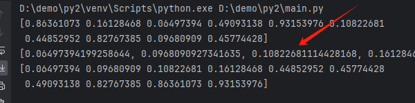
As shown in the figure, using Python’s built-in function can lead to accuracy issues.

Slicing Indexing

You can use the slice(start, stop, step) function or [start:stop:step] for slicing.

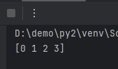
import numpy as np

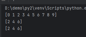
a = np.arange(10)
print(a)

# Index range is 2-7, step is 2
# [0 1 2 3 4 5 6 7 8 9]
s1 = slice(2, 7, 2)

# Index range is 2-8, step is 2
# [0 1 2 3 4 5 6 7 8 9]
s2 = slice(2, 8, 2)

print(a[s1])
print(a[s2])

Equivalent to:

import numpy as np

a = np.arange(10)
print(a)

print(a[2:7:2])
print(a[2:8:2])

For two-dimensional arrays, values can be retrieved using coordinate points.

import numpy as np

x = np.array([[0, 1, 2],
              [3, 4, 5],
              [6, 7, 8],
              [9, 10, 11]])


# Top-left, top-right, bottom-left, bottom-right four points
a1 = np.array([[0, 0], [3, 3]])
a2 = np.array([[0, 2], [0, 2]])

y = x[a1, a2]
print(y)

[[ 0  2]
 [ 9 11]]

When retrieving values, it is consistent with one-dimensional arrays, and can be accessed by index.

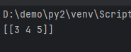
import numpy as np

x = np.array([[0, 1, 2],
              [3, 4, 5],
              [6, 7, 8],
              [9, 10, 11]])

y = x[1:2]
print(y)

Arrays can also be indexed through expressions, like x>5, x<5, etc.

import numpy as np

x = np.array([[0, 1, 2], [3, 4, 5], [6, 7, 8], [9, 10, 11]])
print(x)

print(x[x > 5])

For detailed expression operation methods, refer to the official documentation, and it will not be reiterated here.

Array Operators

Numpy arrays can be manipulated directly using operators.

For example, adding the values of two arrays:

import numpy as np

a1 = np.array([1, 2, 3])
a2 = np.array([4, 5, 6])

a3 = a1 + a2
a4 = a1 * a2
print(a3)
print(a4)

Result in:

[5 7 9]
[ 4 10 18]

Broadcasting Rules

For arrays of different shapes (i.e., different dimensions), numpy can automatically complete the dimensions.

The rules are constrained as follows:

• Two arrays must have the same shape.

• The array with fewer dimensions must be one-dimensional.

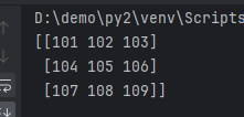
import numpy as np

a = np.array([[1, 2, 3],
              [4, 5, 6],
              [7, 8, 9]])

b = np.array([100, 100, 100])
print(a + b)

[
[1, 2, 3] + [100, 100, 100]
[4, 5, 6] + [100, 100, 100]
[7, 8, 9] + [100, 100, 100]
]

After addition:

[
[101 102 103]
[104 105 106]
[107 108 109]
]

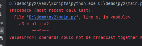
However, it should be noted that if the number of elements in one dimension of the two arrays is inconsistent, an operation error will occur.

import numpy as np

a1 = np.array([1, 2, 3])
a2 = np.array([4, 5, 6, 7])

a3 = a1 + a2
print(a3)

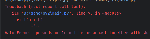
If the two arrays have the same dimensionality but different shapes, the array with fewer dimensions must be one-dimensional.

For example, the following code will report an error:

import numpy as np

a = np.array([[1, 2, 3],
              [1, 1, 1],
              [1, 1, 1]])

b = np.array([[1, 1, 1],
              [2, 2, 2]])
print(a + b)

Modifying Arrays

Numpy contains some functions for handling arrays, which can be roughly divided into the following categories:

• Modifying the shape of an array
• Reversing an array
• Modifying the dimensionality of an array
• Concatenating arrays
• Splitting arrays
• Adding and deleting elements in an array

Modifying the Shape of an Array

The main functions are as follows:

| Function | Description |
| --- | --- |
| reshape | Modify the shape without changing the data |
| flat | Array element iterator |
| flatten | Returns a copy of the array, changes to the copy do not affect the original array |
| ravel | Returns a flattened array |

Converting a one-dimensional array to a two-dimensional array, where each array element has 3 elements, is shown as follows:

import numpy as np

a = np.arange(6).reshape(2, 3)
b = np.array([0, 1, 2, 3, 4, 5]).reshape(2, 3)
print(a)
print(b)

[[0 1 2]
 [3 4 5]]
[[0 1 2]

The other functions can be expressed with the following examples:

import numpy as np

a = np.arange(10)
print(a)

# Array iterator .flat
for element in a.flat:
    print(element)

# Convert the array to a two-dimensional array
b = a.reshape(2, 5)
print("Convert the array to two dimensions:")
print(b)

print("Combine multi-dimensional arrays into one dimension:")
c = b.ravel()
print(c)

[0 1 2 3 4 5 6 7 8 9]
0
1
2
3
4
5
6
7
8
9
Convert the array to two dimensions:
[[0 1 2 3 4]
 [5 6 7 8 9]]
Combine multi-dimensional arrays into one dimension:
[0 1 2 3 4 5 6 7 8 9]

Reversing an Array

Common function definitions are as follows:

| Function | Description |
| :-------------- | :------------------------------- |
| transpose | Swap the dimensions of the array |
| ndarray.T | Same as self.transpose() |
| rollaxis | Roll the specified axis backward |
| swapaxes | Swap two axes of the array |

transpose and ndarray.T can both reverse an array, for example turning a 2x5 array into a 5x2.

import numpy
import numpy as np

a = np.arange(10).reshape(2, 5)
print(a)
b = numpy.transpose(a)
c = a.T
print(b)
print(c)

[[0 1 2 3 4]
 [5 6 7 8 9]]
[[0 5]
 [1 6]
 [2 7]
 [3 8]
 [4 9]]
[[0 5]
 [1 6]
 [2 7]
 [3 8]
 [4 9]]

rollaxis and swapaxes have three parameters:

arr: array
axis: the axis to roll backward, the relative position of other axes will not change. The range is [0, a.ndim]
start: defaults to zero, indicating a complete roll. It can be rolled to a specific position. The range is [-a.ndim, a.ndim]

Note: For two-dimensional arrays, there are only two axes 0 and 1, while for three-dimensional arrays, there are 0, 1, and 2. Both axis and start are entered as the axis numbers.

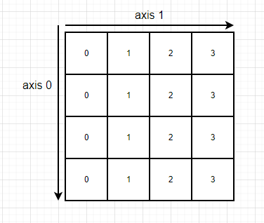
Using print(a1.ndim) can print the dimensionality of the array, which is the number of axes.

swapaxes is used to specify the interaction of the positions of two axes.

For example:

import numpy
import numpy as np

a1 = np.array([
    [0, 0, 0, 0],
    [1, 1, 1, 1],
    [2, 2, 2, 2],
    [3, 3, 3, 3]
])

b = np.swapaxes(a1, 0, 1)

print(b)

Original array:

[[0, 0, 0, 0]
 [1, 1, 1, 1]
 [2, 2, 2, 2]
 [3, 3, 3, 3]]

Transformed array:

[[0 1 2 3]
 [0 1 2 3]
 [0 1 2 3]
 [0 1 2 3]]

It can also be understood as swapping the x-axis and y-axis of a coordinate system, where the x-axis becomes the y-axis.

In the case of more dimensional arrays, swapaxes may have more axes, like the three axes x, y, and z in the three-dimensional case. It will not be detailed further here.

As for numpy.rollaxis, I also do not have knowledge about it.

Modifying the Dimensionality of Arrays

The main functions are as follows:

| Dimensionality | Description |
| :---------------- | :------------------------------- |
| broadcast | Produce an object imitating broadcasting |
| broadcast_to | Broadcast the array to a new shape |
| expand_dims | Expand the shape of the array |
| squeeze | Remove single-dimensional entries from the shape of the array |

Concatenating Arrays

The main functions are as follows:

| Function | Description |
| :---------------- | :----------------------------------- |
| concatenate | Concatenate sequences of arrays along the existing axis |
| stack | Join a series of arrays along a new axis. |
| hstack | Horizontally stack arrays in a sequence (column direction) |
| vstack | Vertically stack arrays in a sequence (row direction) |

numpy.concatenate concatenates two arrays into a new array:

import numpy as np

a = np.array([1, 2, 3, 4])
b = np.array([5, 6, 7, 8])

c = np.concatenate((a, b))
print(c)

Splitting Arrays

The main functions are as follows:

| Function | Array and Operation |
| :----------- | :--------------------------------------- |
| split | Split an array into multiple subarrays |
| hsplit | Split an array horizontally into multiple subarrays (by column) |
| vsplit | Split an array vertically into multiple subarrays (by row) |

The usage method is relatively simple, and will not be repeated here.

Adding and Deleting Elements in Arrays

The main functions are as follows:

| Function | Elements and Description |
| :----------- | :----------------------------------------------- |
| resize | Returns a new array with the specified shape |
| append | Add values to the end of the array |
| insert | Insert values before a specified index along a specific axis |
| delete | Deletes a subarray along a certain axis and returns a new array after deletion |
| unique | Find unique elements within an array |

The usage method is relatively simple and will not be repeated here.

Array Iteration

As previously mentioned, .flat can be used.

import numpy as np

# Here is two-dimensional
a = np.arange(10).reshape(2, 5)

# Array iterator .flat
for element in a.flat:
    print(element)

.flat will print each element in order.

0
1
2
3
4
5
6
7
8
9

.nditer works similarly.

import numpy as np

a = np.arange(10).reshape(2, 5)

# Array iterator .flat
for element in np.nditer(a):
    print(element)

.nditer can control the traversal rules.

for x in np.nditer(a.T, order='C'), by default, traverses by row.

for x in np.nditer(a, order='F'), traverses by column.

import numpy as np

a = np.arange(10).reshape(2, 5)

# Array iterator .flat
for element in np.nditer(a, order='F'):
    print(element)

0
5
1
6
2
7
3
8
4
9

.nditer can control whether to iterate by dimensions or elements.

The previously mentioned code iterates through individual elements.

If flags parameters are set, you can iterate through dimensions.

import numpy as np

a = np.arange(10).reshape(2, 5)

# Array iterator .flat
for element in np.nditer(a, order='F', flags=['external_loop']):
    print(element)

Original array:
[[0 1 2 3 4]
 [5 6 7 8 9]]

Iterated in direction F:
[0 5]
[1 6]
[2 7]
[3 8]
[4 9]