Training and Generating Avatars via Generative Adversarial Networks (GAN)
https://torch.whuanle.cn
E-book repository: https://github.com/whuanle/cs_pytorch
Maomi.Torch project repository: https://github.com/whuanle/Maomi.Torch
Description
This article is adapted from the PyTorch official documentation examples, with some text and images sourced from the PyTorch documentation. Citations are not provided separately at the end of the article.
Official documentation link:
https://pytorch.org/tutorials/beginner/dcgan_faces_tutorial.html
Community Chinese translation version: https://pytorch.ac.cn/tutorials/beginner/dcgan_faces_tutorial.html
PyTorch example project repository:
https://github.com/pytorch/examples
Corresponding Python version example: https://github.com/pytorch/tutorials/blob/main/beginner_source/dcgan_faces_tutorial.py
This project references the dcgan project: https://github.com/whuanle/Maomi.Torch/tree/main/examples/dcgan
Introduction
This tutorial will introduce Generative Adversarial Networks (DCGAN) through an example. In this tutorial, we will train a Generative Adversarial Network (GAN) model to generate new celebrity avatars. Most of the code here is sourced from the DCGAN implementation in pytorch/examples, and the author has ported the code implementation using C#. This document will provide a detailed explanation of the implementation, clarifying how and why the model works. No prior knowledge of GANs is required to read this document; the principles might be somewhat difficult to understand, so it is advisable to follow the approach based on the code.
A generative adversarial network can be simply explained as follows: imagine the author enjoys photography but their skills do not match those of a professional photographer. They practice continuously and show each photo to friends to judge whether it was taken by the author or by a professional. If friends can easily tell it was taken by the author, it indicates there is still room for improvement. The practice continues until friends cannot distinguish whether a picture was taken by the author or a professional. This describes the process of a generative adversarial network.
To design a generative adversarial network, it is necessary to design both a generator and a discriminator. The generator reads training images and trains to transform them into output results, which are then checked by the discriminator, assessing the differences between the generated images and the training images. If the discriminator can tell the difference between the generated images and training images, it indicates more training is required, continuing until the discriminator can no longer distinguish between them.
What is GAN
GANs are a framework that teaches deep learning models to capture the distribution of training data, enabling the generation of new data from the same distribution. GANs were invented by Ian Goodfellow in 2014 and were first described in the paper Generative Adversarial Nets. They consist of two distinct models; one is the generator, and the other is the discriminator. The generator's task is to produce "fake" images that resemble the training images. The discriminator's task is to examine images and output whether they are real training images or fake images from the generator. During training, the generator continuously attempts to fool the discriminator by generating increasingly better fake images while the discriminator strives to become a better detective, accurately classifying real and fake images. The equilibrium point in this game is when the generator produces perfect fake images that seem to come directly from the training data, while the discriminator guesses with 50% confidence whether the generator's output is real or fake.
Now, let's define some symbols that will be used throughout the tutorial, starting with the discriminator. Let $x$ represent the image data. $D(x)$ is the discriminator network that outputs the (scalar) probability that $x$ comes from the training data rather than the generator. Here, since we are dealing with images, the input to $D(x)$ has a size of 3x64x64 (CHW format). Intuitively, when $x$ comes from the training data, $D(x)$ should be high, while when $x$ comes from the generator, $D(x)$ should be low. $D(x)$ can also be thought of as a traditional binary classifier.
For the generator's symbols, let $z$ represent a latent space vector sampled from a standard normal distribution. $G(z)$ denotes the generator function that maps latent vector $z$ to the data space. The goal of $G$ is to estimate the distribution from which the training data originates ($p_{data}$) in order to generate fake samples from that estimated distribution ($p_g$).
Thus, $D(G(z))$ is the probability (scalar) that the generator's output $G$ is a real image. As described in Goodfellow's paper, $D$ and $G$ engage in a min-max game where $D$ tries to maximize the probability of correctly classifying real and fake images ($logD(x)$), while $G$ tries to minimize the probability that $D$ predicts its output as fake ($log(1-D(G(z)))$). In this paper, the GAN loss function is defined as:
$$\underset{G}{\text{min}} \underset{D}{\text{max}}V(D,G) = \mathbb{E}{x\sim p{data}(x)}\big[logD(x)\big] + \mathbb{E}{z\sim p{z}(z)}\big[log(1-D(G(z))\big]$$
Theoretically, the solution to this min-max game is $p_g = p_{data}$, and the discriminator makes random guesses about whether the input is real or fake. However, the convergence theory of GANs is still actively studied, and in practice, the model does not always achieve this point.
What is DCGAN
DCGAN is a direct extension of the above GAN; the difference lies in the explicit use of convolutional layers and deconvolutional layers in both the discriminator and the generator. Radford et al. first described this approach in the paper Unsupervised Representation Learning with Deep Convolutional Generative Adversarial Networks. The discriminator consists of strided convolutional layers, batch normalization layers, and LeakyReLU activation functions. The input is a 3x64x64 input image, and the output is a scalar probability indicating whether the input originates from the real data distribution. The generator comprises transposed convolution layers, batch normalization layers, and ReLU activation functions. The input is a latent vector $z$ drawn from a standard normal distribution, and the output is a 3x64x64 RGB image. The strided transposed convolutional layers allow converting the latent vector into a volume with the same shape as the image. In the paper, the authors also provide suggestions on how to set the optimizer, compute the loss function, and initialize the model weights, which will be explained in subsequent sections.
Next, introduce dependencies and configure training parameters:
using dcgan;
using Maomi.Torch;
using System.Diagnostics;
using TorchSharp;
using TorchSharp.Modules;
using static TorchSharp.torch;

// Start using GPU
Device defaultDevice = MM.GetOpTimalDevice();
torch.set_default_device(defaultDevice);

// Set random seed for reproducibility
var manualSeed = 999;

// manualSeed = random.randint(1, 10000) // use if you want new results
Console.WriteLine("Random Seed:" + manualSeed);
random.manual_seed(manualSeed);
torch.manual_seed(manualSeed);

Options options = new Options()
{
    Dataroot = "E:\\datasets\\celeba",
    // Setting this allows concurrent loading of the dataset, speeding up training
    Workers = 10,
    BatchSize = 128,
};
Later, we will explain how to download the image dataset.
The dataset for training consists of around 220,000 portrait images, making it impractical to load all at once. Therefore, the BatchSize parameter must be set to load and train data in batches. If the reader's GPU performance is high, a larger batch size can be set.
Parameter Explanation
The Options model class defines the parameters for training the model, and below is a detailed explanation of each parameter.
Note that field names may vary slightly, and the ported version does not utilize all parameters.
dataroot- Path to the root directory of the dataset. We will discuss the dataset in detail in the next section.workers- Number of worker threads for loading data withDataLoader.batch_size- Batch size used during training. The DCGAN paper uses a batch size of 128.image_size- The spatial size of the images used for training. This implementation defaults to 64x64. If a different size is required, the structures of D and G must be adjusted. For more details, refer to this link.nc- Number of color channels in the input images. For color images, this value is 3.nz- Length of the latent vector.ngf- Depth of feature maps passed through the generator.ndf- Depth of feature maps passed through the discriminator.num_epochs- The number of training epochs to run. Longer training times may yield better results but will take longer.lr- Learning rate for the training. As stated in the DCGAN paper, this number should be 0.0002.beta1- Beta1 hyperparameter for the Adam optimizer. As stated in the paper, this number should be 0.5.ngpu- Number of available GPUs. If this value is 0, the code will run in CPU mode. If this number is greater than 0, it will run on those GPUs.
First, define a global parameter model class and set default values:
public class Options
{
    /// <summary>
    /// Root directory for dataset
    /// </summary>
    public string Dataroot { get; set; } = "data/celeba";

    /// <summary>
    /// Number of workers for dataloader
    /// </summary>
    public int Workers { get; set; } = 2;

    /// <summary>
    /// Batch size during training
    /// </summary>
    public int BatchSize { get; set; } = 128;

    /// <summary>
    /// Spatial size of training images. All images will be resized to this size using a transformer.
    /// </summary>
    public int ImageSize { get; set; } = 64;

    /// <summary>
    /// Number of channels in the training images. For color images this is 3
    /// </summary>
    public int Nc { get; set; } = 3;

    /// <summary>
    /// Size of z latent vector (i.e. size of generator input)
    /// </summary>
    public int Nz { get; set; } = 100;

    /// <summary>
    /// Size of feature maps in generator
    /// </summary>
    public int Ngf { get; set; } = 64;

    /// <summary>
    /// Size of feature maps in discriminator
    /// </summary>
    public int Ndf { get; set; } = 64;

    /// <summary>
    /// Number of training epochs
    /// </summary>
    public int NumEpochs { get; set; } = 5;

    /// <summary>
    /// Learning rate for optimizers
    /// </summary>
    public double Lr { get; set; } = 0.0002;

    /// <summary>
    /// Beta1 hyperparameter for Adam optimizers
    /// </summary>
    public double Beta1 { get; set; } = 0.5;

    /// <summary>
    /// Number of GPUs available. Use 0 for CPU mode.
    /// </summary>
    public int Ngpu { get; set; } = 1;
}
Dataset Processing
In this tutorial, we will use the Celeb-A Faces dataset to train the model, which can be downloaded from the linked website or from Google Drive.
Official dataset address: https://mmlab.ie.cuhk.edu.hk/projects/CelebA.html
You can download it via Google Drive or Baidu Cloud:
https://drive.google.com/drive/folders/0B7EVK8r0v71pWEZsZE9oNnFzTm8?resourcekey=0-5BR16BdXnb8hVj6CNHKzLg&usp=sharing
https://pan.baidu.com/s/1CRxxhoQ97A5qbsKO7iaAJg
Extraction code:
rp0s
Note that this tutorial only requires the images and does not require the labels. It is unnecessary to download all files; just download CelebA/Img/img_align_celeba.zip. After downloading, extract it to an empty directory, with a sample directory structure as follows:
/path/to/celeba
    -> img_align_celeba
        -> 188242.jpg
        -> 173822.jpg
        -> 284702.jpg
        -> 537394.jpg
           ...
Then specify /path/to/celeba in the Options.Dataroot parameter. The dataset will automatically search the subdirectories within this directory and treat them as classification names for images, loading all image files from the subdirectories.
This is an important step because we will use the ImageFolder dataset class, which requires that the root folder of the dataset contains subdirectories. Now we can create the dataset, create a data loader, set the running device, and finally visualize some training data.
// Create a samples directory to output the results produced during training
if (Directory.Exists("samples"))
{
    Directory.Delete("samples", true);
}

Directory.CreateDirectory("samples");

// Load images and perform transformations
var dataset = MM.Datasets.ImageFolder(options.Dataroot, torchvision.transforms.Compose(
    torchvision.transforms.Resize(options.ImageSize),
    torchvision.transforms.CenterCrop(options.ImageSize),
    torchvision.transforms.ConvertImageDtype(ScalarType.Float32),
    torchvision.transforms.Normalize(new double[] { 0.5, 0.5, 0.5 }, new double[] { 0.5, 0.5, 0.5 }))
);

// Load images in batches
var dataloader = torch.utils.data.DataLoader(dataset, batchSize: options.BatchSize, shuffle: true, num_worker: options.Workers, device: defaultDevice);

var netG = new dcgan.Generator(options).to(defaultDevice);
After setting the input parameters and preparing the dataset, we can now proceed to the implementation part. We will begin with weight initialization strategies, followed by detailed discussions on the generator, discriminator, loss functions, and training loops.
Weight Initialization
According to the DCGAN paper, all model weights should be randomly initialized from a normal distribution with a mean of 0 and a standard deviation of 0.02. The weights_init function takes an initialized model as input and re-initializes all convolutional layers, transposed convolutional layers, and batch normalization layers to meet this standard. This function is applied to the model immediately after initialization.
static void weights_init(nn.Module m)
{
    var classname = m.GetType().Name;
    if (classname.Contains("Conv"))
    {
        if (m is Conv2d conv2d)
        {
            nn.init.normal_(conv2d.weight, 0.0, 0.02);
        }
    }
    else if (classname.Contains("BatchNorm"))
    {
        if (m is BatchNorm2d batchNorm2d)
        {
            nn.init.normal_(batchNorm2d.weight, 1.0, 0.02);
            nn.init.zeros_(batchNorm2d.bias);
        }
    }
}
The network model will have multiple layers, and the weights_init function will automatically be called at different layers during model training. The target objects are not the model itself but the layers of the network model.
Generator
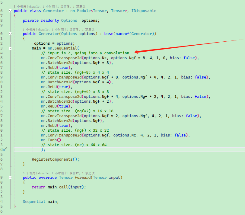
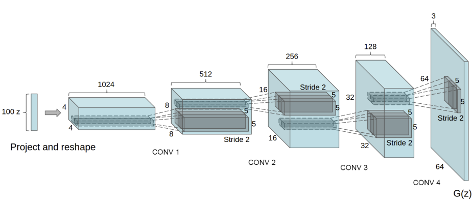
The generator $G$ aims to map latent space vectors ($z$) to data space. Since our data comprises images, converting $z$ to data space means ultimately creating an RGB image of the same size as the training images (i.e., 3x64x64). In practice, this is achieved through a series of 2D transposed convolutional layers, each equipped with a 2D batch normalization layer and a ReLU activation function. The output of the generator is returned to the input data range $[-1,1]$ via a tanh function. Notably, a batch normalization function follows the conv-transpose layers, as this is one of the significant contributions of the DCGAN paper. These layers help with the flow of gradients during training. The diagram below shows the generator from the DCGAN paper.
Note how the input settings (nz, ngf, and nc) affect the code architecture of the generator. nz is the length of the z input vector, ngf relates to the size of feature maps propagated in the generator, while nc denotes the number of channels in the output image (set to 3 for RGB images). Below is the code for the generator.
.
Defining the network model for image generation:
public class Generator : nn.Module<Tensor, Tensor>, IDisposable
{
    private readonly Options _options;

    public Generator(Options options) : base(nameof(Generator))
    {
        _options = options;
        main = nn.Sequential(
            // input is Z, going into a convolution
            nn.ConvTranspose2d(options.Nz, options.Ngf * 8, 4, 1, 0, bias: false),
            nn.BatchNorm2d(options.Ngf * 8),
            nn.ReLU(true),
            // state size. (ngf*8) x 4 x 4
            nn.ConvTranspose2d(options.Ngf * 8, options.Ngf * 4, 4, 2, 1, bias: false),
            nn.BatchNorm2d(options.Ngf * 4),
            nn.ReLU(true),
            // state size. (ngf*4) x 8 x 8
            nn.ConvTranspose2d(options.Ngf * 4, options.Ngf * 2, 4, 2, 1, bias: false),
            nn.BatchNorm2d(options.Ngf * 2),
            nn.ReLU(true),
            // state size. (ngf*2) x 16 x 16
            nn.ConvTranspose2d(options.Ngf * 2, options.Ngf, 4, 2, 1, bias: false),
            nn.BatchNorm2d(options.Ngf),
            nn.ReLU(true),
            // state size. (ngf) x 32 x 32
            nn.ConvTranspose2d(options.Ngf, options.Nc, 4, 2, 1, bias: false),
            nn.Tanh()
            // state size. (nc) x 64 x 64
            );

        RegisterComponents();
    }

    public override Tensor forward(Tensor input)
    {
        return main.call(input);
    }

    Sequential main;
}
Initializing the model:
var netG = new dcgan.Generator(options).to(defaultDevice);
netG.apply(weights_init);
Console.WriteLine(netG);
Discriminator
As mentioned earlier, the discriminator $D$ is a binary classification network that takes an image as input and outputs a scalar probability, representing the likelihood that the input image is real (rather than fake). Here, $D$ accepts a 3x64x64 input image and processes it through a series of Conv2d, BatchNorm2d, and LeakyReLU layers, ultimately outputting the final probability through a Sigmoid activation function. This architecture can be extended to include more layers as necessary, but it makes sense to use strided convolutions, BatchNorm, and LeakyReLUs. The DCGAN paper suggests that using strided convolutions instead of pooling for downsampling is a good practice because it allows the network to learn its own pooling function. Additionally, batch normalization and the leaky ReLU function promote healthy gradient flow, which is crucial for the learning process of both $G$ and $D$.
Defining the discriminator network model:
public class Discriminator : nn.Module<Tensor, Tensor>, IDisposable
{
    private readonly Options _options;

    public Discriminator(Options options) : base(nameof(Discriminator))
    {
        _options = options;

        main = nn.Sequential(
            // input is (nc) x 64 x 64
            nn.Conv2d(options.Nc, options.Ndf, 4, 2, 1, bias: false),
            nn.LeakyReLU(0.2, inplace: true),
            // state size. (ndf) x 32 x 32
            nn.Conv2d(options.Ndf, options.Ndf * 2, 4, 2, 1, bias: false),
            nn.BatchNorm2d(options.Ndf * 2),
            nn.LeakyReLU(0.2, inplace: true),
            // state size. (ndf*2) x 16 x 16
            nn.Conv2d(options.Ndf * 2, options.Ndf * 4, 4, 2, 1, bias: false),
            nn.BatchNorm2d(options.Ndf * 4),
            nn.LeakyReLU(0.2, inplace: true),
            // state size. (ndf*4) x 8 x 8
            nn.Conv2d(options.Ndf * 4, options.Ndf * 8, 4, 2, 1, bias: false),
            nn.BatchNorm2d(options.Ndf * 8),
            nn.LeakyReLU(0.2, inplace: true),
            // state size. (ndf*8) x 4 x 4
            nn.Conv2d(options.Ndf * 8, 1, 4, 1, 0, bias: false),
            nn.Sigmoid()
            );

        RegisterComponents();
    }

    public override Tensor forward(Tensor input)
    {
        var output =  main.call(input);

        return output.view(-1, 1).squeeze(1);
    }

    Sequential main;
}
Initializing the model:
var netD = new dcgan.Discriminator(options).to(defaultDevice);
netD.apply(weights_init);
Console.WriteLine(netD);
Loss Function and Optimizer
After setting up $D$ and $G$, we can specify their learning method through the loss function and optimizers. We will use the binary cross-entropy loss function (BCELoss), which is defined in PyTorch as follows:
$$
\ell(x, y) = L = {l_1,\dots,l_N}^\top, \quad l_n = - \left[ y_n \cdot \log x_n + (1 - y_n) \cdot \log (1 - x_n) \right]
$$
Note that this function provides the calculation for the two log components in the objective function, namely $log(D(x))$ and $log(1-D(G(z)))$. We can specify which part of the BCE equation to use via the $y$ input. This will be accomplished in the upcoming training loop, but it is important to understand that we can choose which component we wish to compute by changing $y$ (i.e., GT labels).
Next, we will define real labels as 1 and fake labels as 0. These labels will be used when computing the losses for $D$ and $G$, which is also a convention used in the original GAN paper. Finally, we set up two independent optimizers, one for $D$ and another for $G$. According to the DCGAN paper, both are Adam optimizers with a learning rate of 0.0002 and Beta1 = 0.5. To track the generator's learning progress, we will generate a fixed batch of latent vectors drawn from a Gaussian distribution (i.e., fixed_noise). During the training loop, we will periodically input this fixed_noise into $G$, and we will see the images being formed from noise over the iterations.
var criterion = nn.BCELoss();
var fixed_noise = torch.randn(new long[] { options.BatchSize, options.Nz, 1, 1 }, device: defaultDevice);
var real_label = 1.0;
var fake_label = 0.0;
var optimizerD = torch.optim.Adam(netD.parameters(), lr: options.Lr, beta1: options.Beta1, beta2: 0.999);
var optimizerG = torch.optim.Adam(netG.parameters(), lr: options.Lr, beta1: options.Beta1, beta2: 0.999);
Training
Finally, after we have defined all the components of the GAN framework, we can commence training it. Note that training GANs is somewhat of an art, as improper hyper-parameter settings can lead to mode collapse and it can be difficult to diagnose what the problem is. Here, we will closely follow the algorithm from Goodfellow's paper as Algorithm 1, while also adhering to some best practices shown in ganhacks. Specifically, we will “construct different mini-batches for real and fake images” and adjust the objective function for $G$ to maximize $log(D(G(z)))$. The training process is divided into two main parts: the first part updates the discriminator, and the second part updates the generator.
Part 1 - Training the Discriminator
To summarize, the goal of training the discriminator is to maximize the probability of correctly classifying the given input as real or fake. According to Goodfellow, we aim to “update the discriminator by ascending random gradients.” In practice, we want to maximize $log(D(x)) + log(1-D(G(z)))$. Following the independent mini-batch recommendations from ganhacks, we will compute this in two steps. First, we will construct a mini-batch of real samples from the training set, perform a forward pass through $D$, compute the loss ($log(D(x))$), and then backpropagate to compute the gradients. Second, we will use the current generator to construct a mini-batch of fake samples, perform a forward pass through $D$, compute the loss ($log(1-D(G(z)))$), and backpropagate to accumulate the gradients. Now, with the gradients accumulated from both the all-real and all-fake batches, we will take a step with the discriminator optimizer.
Part 2 - Training the Generator
As stated in the original paper, we wish to train the generator by minimizing $log(1-D(G(z)))$ to produce better fake samples. As previously mentioned, Goodfellow showed this does not provide sufficient gradient early in the learning process. As a solution, we want to maximize $log(D(G(z)))$. In code, we achieve this by classifying the output from the generator of the first part using the discriminator, using real labels as GT to compute the loss for $G$, calculating the gradients for $G$ during backpropagation, and finally taking a step to update the parameters of $G$ with the optimizer. Using real labels as the GT labels for the loss function may seem counterintuitive, but it allows us to use the $log(x)$ component of BCELoss (rather than the $log(1-x)$ component), which is exactly what we need.
Finally, we will report some statistics and at the end of each epoch, we will push our fixed noise batch through the generator to visually track the training progress of $G$. The reported training statistics include:
- Loss_D - Discriminator loss, computed as the sum of losses for the all-real and all-fake batches ($log(D(x)) + log(1 - D(G(z)))$).
- Loss_G - Generator loss, computed as $log(D(G(z)))$.
- D(x) - Average output of the discriminator for the all-real batch (across batches). This should start near 1 and theoretically converge to 0.5 as $G$ improves. Think about why this is the case.
- D(G(z)) - Average output of the discriminator for the all-fake batch. The first number is before the update of $D$, while the second number is after the update. These numbers should start near 0 and converge to 0.5 as $G$ improves. Think about why this is the case.
Note: This step may take some time, depending on how many epochs you run and whether you remove some data from the dataset.
var img_list = new List<Tensor>();
var G_losses = new List<double>();
var D_losses = new List<double>();

Console.WriteLine("Starting Training Loop...");

Stopwatch stopwatch = new();
stopwatch.Start();
int i = 0;
// For each epoch
for (int epoch = 0; epoch < options.NumEpochs; epoch++)
{
    foreach (var item in dataloader)
    {
        var data = item[0];

        netD.zero_grad();
        // Format batch
        var real_cpu = data.to(defaultDevice);
        var b_size = real_cpu.size(0);
        var label = torch.full(new long[] { b_size }, real_label, dtype: ScalarType.Float32, device: defaultDevice);
        // Forward pass real batch through D
        var output = netD.forward(real_cpu);
        // Calculate loss on all-real batch
        var errD_real = criterion.call(output, label);
        // Calculate gradients for D in backward pass
        errD_real.backward();
        var D_x = output.mean().item<float>();

        // Train with all-fake batch
        // Generate batch of latent vectors
        var noise = torch.randn(new long[] { b_size, options.Nz, 1, 1 }, device: defaultDevice);
        // Generate fake image batch with G
        var fake = netG.call(noise);
        label.fill_(fake_label);
        // Classify all fake batch with D
        output = netD.call(fake.detach());
        // Calculate D's loss on the all-fake batch
        var errD_fake = criterion.call(output, label);
        // Calculate the gradients for this batch, accumulated (summed) with previous gradients
        errD_fake.backward();
        var D_G_z1 = output.mean().item<float>();
        // Compute error of D as sum over the fake and the real batches
        var errD = errD_real + errD_fake;
        // Update D
        optimizerD.step();

        ////////////////////////////
        // (2) Update G network: maximize log(D(G(z)))
        ////////////////////////////
        netG.zero_grad();
        label.fill_(real_label);  // fake labels are real for generator cost
        // Since we just updated D, perform another forward pass of all-fake batch through D
        output = netD.call(fake);
        // Calculate G's loss based on this output
        var errG = criterion.call(output, label);
        // Calculate gradients for G
        errG.backward();
        var D_G_z2 = output.mean().item<float>();
        // Update G
        optimizerG.step();

        // ex: [0/25][4/3166] Loss_D: 0.5676 Loss_G: 7.5972 D(x): 0.9131 D(G(z)): 0.3024 / 0.0007
        Console.WriteLine($"[{epoch}/{options.NumEpochs}][{i%dataloader.Count}/{dataloader.Count}] Loss_D: {errD.item<float>():F4} Loss_G: {errG.item<float>():F4} D(x): {D_x:F4} D(G(z)): {D_G_z1:F4} / {D_G_z2:F4}");

        // Every 100 batches, output an image effect
        if (i % 100 == 0)
        {
            real_cpu.SaveJpeg("samples/real_samples.jpg");
            fake = netG.call(fixed_noise);
            fake.detach().SaveJpeg($"samples/fake_samples_epoch_{epoch:D3}.jpg");
        }

        i++;
    }


    netG.save($"samples/netg_{epoch}.dat");
    netD.save($"samples/netd_{epoch}.dat");
}
Finally, print the training results and output:
Console.WriteLine("Training finished.");
stopwatch.Stop();
Console.WriteLine($"Training Time: {stopwatch.Elapsed}");

netG.save("samples/netg.dat");
netD.save("samples/netd.dat");
According to the official example recommendations, 25 epochs of training were performed. Due to the author using a 4060TI 8G machine for training, the estimated time for 25 epochs is:
Training finished.
Training Time: 00:49:45.6976041
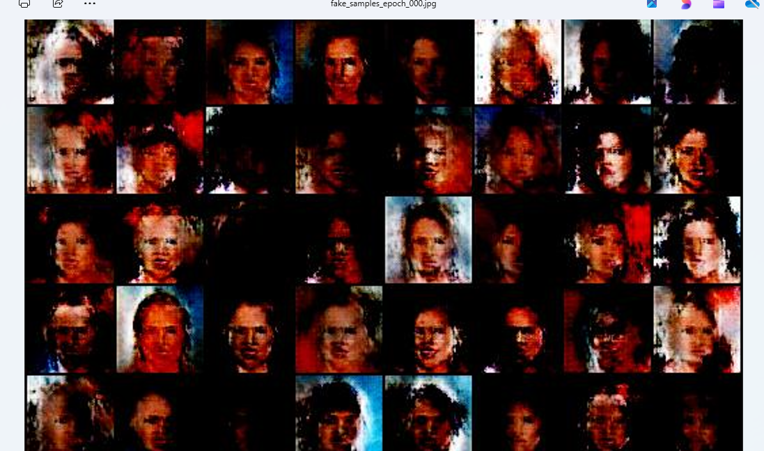
Images from each epoch of training:
First epoch generation:
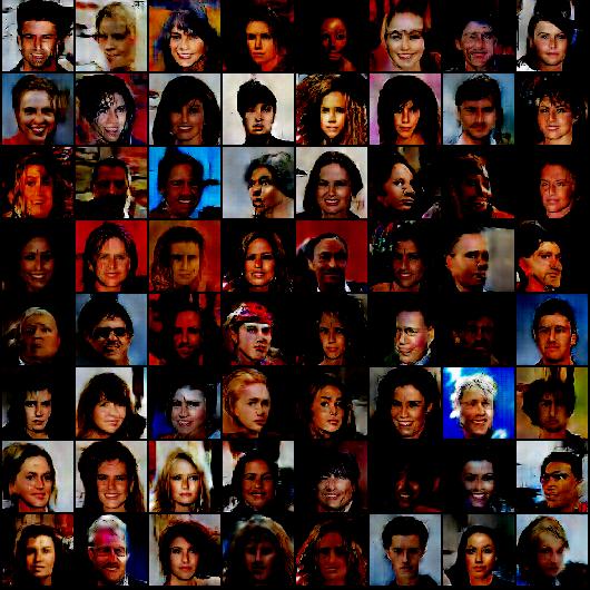
The generation from the 25th epoch:
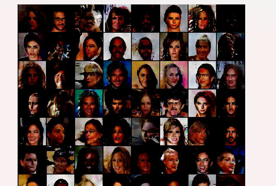
Although it is still somewhat abstract, the generated results are better than before.
In the dcgan_out project, I saw the model output from the 5 epochs of training generating images:
Device defaultDevice = MM.GetOpTimalDevice();
torch.set_default_device(defaultDevice);

// Set random seed for reproducibility
var manualSeed = 999;

// manualSeed = random.randint(1, 10000) # use if you want new results
Console.WriteLine("Random Seed:" + manualSeed);
random.manual_seed(manualSeed);
torch.manual_seed(manualSeed);


Options options = new Options()
{
    Dataroot = "E:\\datasets\\celeba",
    Workers = 10,
    BatchSize = 128,
};

var netG = new dcgan.Generator(options);
netG.to(defaultDevice);
netG.load("netg.dat");

// Generate random noise
var fixed_noise = torch.randn(64, options.Nz, 1, 1, device: defaultDevice);

// Generate images
var fake_images = netG.call(fixed_noise);

fake_images.SaveJpeg("fake_images.jpg");
Although it is still somewhat abstract, it is indeed quite good.

文章评论